5. Probability Distributions

We have seen how it is possible to assign a probability value to a given outcome of a random variable.

In practice, it is often useful to assign probability values to all the values that the random variable can assume.

To do so, we can define a function, which we will call probability distribution which assigns a probability value to each of the possible values of a random variable.

In the case of discrete variables, we will talk about “probability mass functions”, whereas in the case of continuous variable, we will refer to “probability density functions”.

A probability distribution characterizes the random variable and defines which outcomes it is more likely to observe.

Once we find that a given random variable \(X\) is characterized by a probability distirbution \(P(X)\), we can say that “X follows P” and write:

\[X \sim P\]

5.1. Probability Mass Functions (PMF) - Discrete Variables

If \(X\) is discrete, \(P(X)\) is called a “probability mass function” (PMF). \(P\) maps the values of \(X\) to real numbers indicating whether a given value is more or less likely.

A PMF on a random variable \(X\) is a function

\[P:\Omega \rightarrow \lbrack 0,1\rbrack\]

Where \(\Omega\) is the sample space \(X\), which satisfies the following property:

\[\sum_{\mathbf{x}\mathbf{\in}\mathbf{\Omega}}^{}{\mathbf{P}\mathbf{(}\mathbf{x}\mathbf{)}}\mathbf{=}\mathbf{1}\]

This condition implies that the probability distribution is normalized. Also, this means that at least one of the events should happen.

Example: Let \(X\) be the random variable indicating the outcome of a coin toss.

• The space of all possible functions (the domain of \(P(X)\)) is \(\{ head,\ tail\}\).

• The probabilities \(P(head)\) and \(P(tail)\) must be larger than or equal to zero and smaller than or equal to 1.

• Also, \(P(head) + P(tail) = 1\ \). This is obvious, as one of the two outcomes will always happen. Indeed, if we had \(P(tail) = 0.3\), this would mean that, 30 times out of 100 times we toss a coin, the outcome will be tail. What will happen in all other cases? The outcome will be head, hence, \(P(head)\), so \(P(head) + P(tail) = 1\).

• In the case of a fair coin, we can characterize \(P(X)\) as a “discrete uniform distribution”, i.e., a distribution which maps any value \(x \in X\) to a constant, such that the properties of the probability mass functions are satisfied.

• If we have \(N\) possible outcomes, the discrete uniform probability will be \(P(X = x) = \frac{1}{N}\) , which means that all outcomes have the same probability.

• This definition satisfies the constraints. Indeed, \(\frac{1}{N} \geq 0,\ \forall N\) and \(\sum_{i}^{}{P\left( X = x_{i} \right)} = 1\).

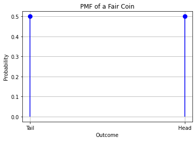
5.1.1. Example: Probability Mass Function for a Fair Coin

A probability mass function can be plotted as a 2D diagram where the values of the function (\(P(x)\)) is plotted against the values of the independent variable \(x\). This is the diagram associated to the PMF of the previous example, where \(P(head) = P(tail) = 0.5\).

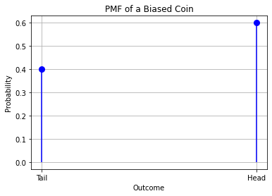
5.1.2. Example: Probability Mass Function for a Biased Coin

Now suppose we tossed our coin for 10000 times and discovered that 6000 times the outcome was “head”, whereas 4000 times it was “tail”. We deduce the coin is not fair.

Using a frequentist approach, we can manually assign values to our PMF using the general formula:

\[P(x) = \frac{\# trials\ in\ which\ X = x}{\#\ trials}\]

That is, in our case:

\[P(head) = \frac{6000}{10000} = 0.6;P(tail) = \frac{4000}{10000} = 0.4\]

We shall note that the probability we just defined satisfies all properties of probabilities, i.e.:

• \(0 \leq P(x) \leq 1\ \forall x\)

• \(\sum_{x}^{}{P(x) = 1}.\)

5.1.2.1. Exercise: Probability Mass Function

Let \(X\) be a random variable representing the outcome of rolling a fair dice with \(6\) faces:

• What is the space of possible values of \(X\)?

• What is its cardinality?

• What is the associated probability mass function \(P(X)\)?

• Suppose the dice is not fair and \(P(X = 1) = 0.2\), whereas all other outcomes are equally probable. What is the probability mass function of \(P(X)\)?

• Draw the PMF obtained for the dice.

5.2. Probability Density Functions (PDF) - Continuous Variables

Probability distributions are called “probability density functions” when the random variable is continuous.

A probability density function over a variable \(X\) is defined as follows:

\[f:\Omega \rightarrow \lbrack 0,1\rbrack\]

and must satisfy the following property:

\[\int f(x)dx = 1\]

This condition is equivalent to \(\sum P(x) = 1\) in the case of a discrete variable. The sum turns into an integral in the case of continuous variables.

Note that, in the case of continuous variables, we have:

\[ P(a \leq x \leq b) = \int_{a}^b f(x) dx\]

NOTE: In general, we say that the density function at a given value \(x\) is zero: \(f(x)=0\). While this may seem counter-intuitive, we should consider the density function as the limit fo the probability as we narrow a neighborhood around \(x\). If the neighborhood has size \(0\), then the density will be zero. In practice, if we take a neighborhood which is non-zero, then we get an integral between two values and a final probability not equal to zero.

After all, from an intuitive point of view, the probability of having a value exactly equal to \(x\) is indeed zero, in the case of a continuous variable! So we should be more interested in the probability in a given range of values.

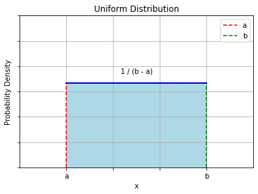
5.2.1. Example: Uniform PDF

Let us consider a random number generator which outputs numbers comprised between \(a\) and \(b\).

Let \(X\) be a random variable assuming the values generated by the random number generator.

The PDF of \(X\) will be a uniform distribution such that:

• \(P(x) = 0\ \forall x < a\ \ or\ x > b\);

• \(P(x) = \frac{1}{b - a}\ \forall a \leq x \leq b\);

We can see that this PDF satisfies all constraints:

• \(P(x) \geq 0\ \forall x.\)

• \(\int P(x)dx = 1\) (prove that this is true as an exercise).

The diagram below shows an illustration of a uniform PDF with bounds a and b, i.e., \(U(a,b)\). Of course, continuous distributions can be (and generally are) much more complicated than that.

5.2.2. Cumulative Distribution Functions (CDF)

Similar to the Empirical Cumulative Distribution Functions, we can define Cumulative Distribution Functions for random variables, starting from the density or mass functions. A cumulative distribution function is generally defined as:

\[ F(x) = f(X \leq x) \]

5.2.3. CDF of Continuous Random Variables

In the case of continuous random variables, the definition leads to:

\[F(x) = \int_{-\infty}^x P(x)dx\]

The CDF is useful in different ways. For instance, it’s easy to see that:

\[P(a \leq X \leq b) = \int_a^b f(x)dx = \int_{-\infty}^b f(x)dx - \int_{-\infty}^a f(x)dx = F(b) - F(a)\]

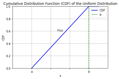
5.2.4. Example

The CDF of the uniform distribution will be given by:

• \(F(x) = 0\) for \(x < a\)

• \(F(x) = \frac{x - a}{b - a}\) for \(a \leq x \leq b\)

• \(F(x) = 1\) for \(x > b\)

The plot below shows a diagram:

5.2.5. CDF of Discrete Random Variables

In the case of discrete random variables, the definition of CDF leads to:

\[F(x) = \sum_{y\leq x} P(y)\]

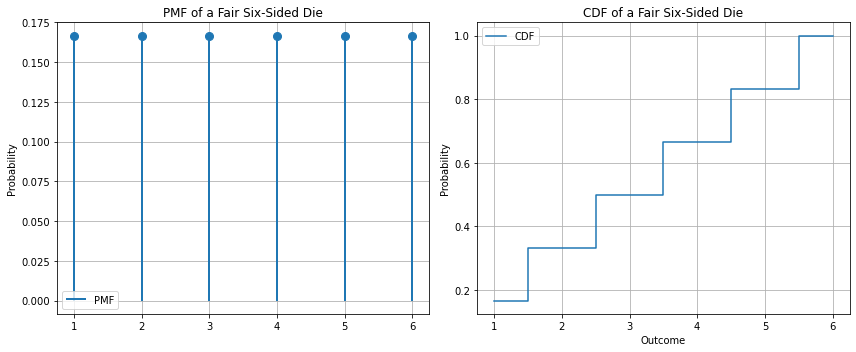
5.2.5.1. Example - PDF and CDF of a fair die

In the case of a fair die, the PMF will be:

\[\begin{split} f(x) = \begin{cases} \frac{1}{6} & \text{if } x \in \{1, 2, 3, 4, 5, 6\} \\ 0 & \text{otherwise} \end{cases} \end{split}\]

The CDF will be:

\[\begin{split} F(x) = \begin{cases} 0 & \text{if } x < 1 \\ \frac{1}{6} & \text{if } 1 \leq x < 2 \\ \frac{1}{3} & \text{if } 2 \leq x < 3 \\ \frac{1}{2} & \text{if } 3 \leq x < 4 \\ \frac{2}{3} & \text{if } 4 \leq x < 5 \\ 1 & \text{if } x \geq 5 \end{cases} \end{split}\]

The diagram below shows an example:

5.3. Expectation

When it is known that a random variable follows a probability distribution, it is possible to characterize that variable (and hence the related probability distribution) with some statistics.

The most straightforward of them is the expectation. The concept of expectation is very related to the concept of mean. When we compute the mean of a given set of numbers, we usually sum all the numbers together and then divide by the total.

Since a probability distribution will tell us which values will be more frequent than others, we can compute this mean with a weighted average, where the weights are given by the probability distribution.

Specifically, we can define the expectation of a random variable X as follows:

\[E_{X\sim P}\lbrack X\rbrack = \sum_{x \in \chi}^{}{xP(x)}\]

In the case of continuous variables, the expectation takes the form of an integral:

\[E_{X \sim P}\lbrack X\rbrack = \int xf(x)dx\]

This is very related to the concept of mean value (or expected value) of a random variable.

5.4. Variance

The variance gives a measure of how much variability there is in a variable \(X\) around its mean \(E\lbrack X\rbrack\).

The variance is defined as follows:

\[var\lbrack X\rbrack = E\lbrack\left( X - E\lbrack X\rbrack \right)^{2}\rbrack\]

5.5. Covariance

The covariance gives a measure of how two variables are linearly related to each other. It allows to measure to what extent the increase of one of the variables corresponds to an increase of the value of the other one.

Given two random variables \(X\) and \(Y\), the covariance is defined as follows:

\[Cov(X,Y) = E\lbrack\left( X - E\lbrack X\rbrack \right)\left( Y - E\lbrack Y\rbrack \right)\rbrack\]

We can distinguish the following terms:

• \(E\lbrack X\rbrack\) and \(E\lbrack Y\rbrack\) are the expectations of \(X\) and \(Y.\)

• \((X - E\lbrack X\rbrack)\) and \((Y - E\lbrack Y\rbrack)\) are the differences between the samples and the expected values.

• \(\left( X - E\lbrack X\rbrack \right)\left( Y - E\lbrack Y\rbrack \right)\) computes the product between the differences.

We have:

• If the signs of the terms agree, the product is positive.

• If the signs of the terms disagree, the product is negative.

In practice, if when \(X\) is larger than the mean, then \(Y\) is larger than the mean and vice versa, when \(X\) is lower than the mean then \(Y\) is lower than the mean, then the two variables are correlated, and the covariance is high.

If \(X\) is a multi-dimensional variable \(X = \lbrack X_{1},X_{2},\ldots,X_{n}\rbrack\), we can compute all the possible covariances between variable pairs: \(Cov\lbrack X_{i},X_{j}\rbrack\). This allows to create a matrix, which is generally referred to as the covariance matrix. The general term of the covariance matrix \(Cov(X)\) is given by:

\[Cov(X)_{i,j} = \Sigma_{ij} = Cov(X_{i},X_{j})\]

5.6. Standardization

Standardization transforms a random variable \(X\) into a variable \(Z\) so that it has:

• Expectation equal to zero: \(E(Z) = 0\).

• Variance equal to one: \(Var(Z) = 1\).

The standardized variable will be:

\[Z = \frac{X - \mu_X}{\sigma_X} = \frac{X-E[X]}{\sqrt{Var[X]}}\]

5.7. Common Probability Distributions

There are several common probability distributions which can be used to describe random events. These distributions have an analytical formulation which depends generally on one or more parameters.

When we have enough evidence that a given random variable is well described by one of these distributions, we can simply “fit” the distribution to the data (i.e., choose the correct parameters for the distribution) and use the analytical formulation to deal with the random variable.

It is hence useful to know the most common probability distributions so that we can recognize the cases in which they can be used.

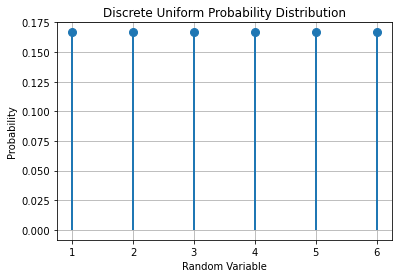
5.7.1. Discrete Uniform Distribution

The discrete uniform distribution is controlled by a parameter \(k \in \mathbb{N}\) and assumes that all outcomes have the same probability of occurring:

\[P(X=a_i) = \frac{1}{k}\]

Where \(\Omega = \{a_1,\ldots,a_k\}\).

It can be shown that:

\[E[X] = \frac{k+1}{2}\]

\[Var[X] = \frac{1}{12}(k^2-1)\]

5.7.1.1. Example

The outcomes of rolling a fair die follow a uniform distribution with \(k=6\), as shown in the diagram below:

5.7.2. Bernoulli Distribution

The Bernoulli distribution is a distribution over a single binary random variable, i.e., the variable \(X\) can take only two values: \(\left\{ 0,1 \right\}\).

The distribution is controlled by a single parameter \(\phi \in \lbrack 0,1\rbrack\), which gives the probability of the variable to be equal to 1.

The analytical formulation of the Bernoulli distribution is very simple:

• \(P(X = 1) = \phi\);

• \(P(X = 0) = 1 - \phi\)

The expected value and variance of the associated random variable are:

• \(E\lbrack x\rbrack = \phi\);

• \(Var(x) = \phi(1 - \phi)\).

5.7.2.1. Example

A skewed coin lands on “head” \(60\%\) of the times. If we define \(X = 1\) when the outcome is head and \(X = 0\) when the outcome is tail, then the variable follows a Bernoulli distribution with \(\phi = 0.6\).

5.7.3. Binomial Distribution

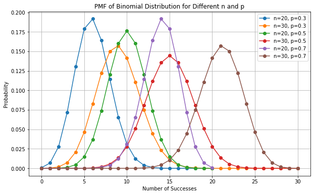
The binomial distribution is a discrete probability distribution (PMF) over natural numbers with parameters \(\mathbf{n}\) and \(\mathbf{p}\)

It models the probability of obtaining \(\mathbf{k}\) successes in a sequence of \(\mathbf{n}\) independent experiments which follow a Bernoulli distribution with parameter \(\mathbf{p}\mathbf{\ (}\mathbf{\phi}\mathbf{=}\mathbf{p}\mathbf{)}\);

The probability mass function of the distribution is given by:

\[P(k) = \binom{n}{k}p^{k}(1 - p)^{n - k}\]

Where:

• \(k\) is the number of successes

• \(n\) is the number of independent trials

• \(p\) is the probability of a success in a single trial

The expected value is \(E\lbrack k\rbrack = np\);

The variance is \(Var\lbrack k\rbrack = np(1 - p)\);

5.7.3.1. Example

What is the probability of tossing a coin three times and obtaining three heads? We have:

• \(k = 3\): number of successes (three times head)

• \(n = 3\): number of trials

• \(p = 0.5\): the probability of getting a head when tossing a coin

The required probability will be given by:

\[P(3) = \binom{3}{3}{0.5}^{3}(1 - 0.5)^{3 - 3} = {0.5}^{3} = 0.125\]

Exercise

What is the probability of tossing an unfair coin (\(P\left( 'head^{'} \right) = 0.6\)) 7 times and obtaining \(2\) tails?

5.7.4. Categorical Distribution

The multinoulli or categorical distribution is a distribution of a single discrete variable with \(k\) different states, where \(k\) is finite.

• The distribution is parametrized by a vector \(\mathbf{p} \in \lbrack 0,1\rbrack^k\), where \(p_{i}\) gives the probability of the \(i^{th}\) state.

• \(\mathbf{p}\) must be such that \(\sum_{i = 1}^kp_{i} = 1\) to obtain a valid probability distribution.

• The analytical form of the distribution is given by: \(p(x = i) = p_{i}\);

This distribution is the generalization of the Bernoulli distribution to the case of multiple states.

Example:

Rolling a fair die. In this case, \(k = 6\) and \(p_{i} = \frac{1}{k}\ ,\ i = 0,\ldots,k \ \).

5.7.5. Multinomial Distribution

The multinomial distribution generalizes the binomial distribution to the case in which the experiments are not binary, but they can have multiple outcomes (e.g., a dice vs a coin).

In particular, the multinomial distribution models the probability of obtaining exactly \((n_{1},\ldots,n_{k})\) occurrences (with \(n = \sum_{i}^{}n_{i}\)) for each of the \(k\) possible outcomes in a sequence of \(n\) independent experiments which follow a Categorial distribution with probabilities \(p_{1},\ldots,p_{k}\).

The parameters of the distribution are:

• \(n\): the number of trials

• \(k\): the number of possible outcomes

• \(p_{1},\ldots,p_{k}\) the probabilities of obtaining a given class in each trial (with \(\sum_{i = 1}^{k}p_{i} = 1\))

The PMF of the distribution is:

\[P\left( n_{1},\ldots,n_{k} \right) = \frac{n!}{n_{1}!\ldots n_{k}!}p_{1}^{n_{1}} \cdot \ldots \cdot p_{k}^{n_{k}}\]

The mean is: \(E\left\lbrack n_{i} \right\rbrack = np_{i}\).

The variance is: \(Var\left\lbrack n_{i} \right\rbrack = np_{i}(1 - p_{i})\).

The covariance between two of the input variables is: \(Cov\left( n_{i},n_{j} \right) = - np_{i}p_{j}\ (i \neq j)\).

Example

Given a fair die with 6 possible outcomes, what is the probability of getting 3 times 1, 2 times 2, 4 time 3, 5 times 4, 0 times 5, and 1 time 6, rolling the dice for 15 times?

We have:

• \(n = 15\)

• \(k = 6\)

• \(p_{1} = p_{2} = \ldots p_{6} = \frac{1}{6}\)

The required probability is given by:

\[P(3,2,4,5,0,1) = \frac{15!}{3!2!4!5!0!1!} \cdot \frac{1}{6^{3}} \cdot \frac{1}{6^{2}} \cdot \frac{1}{6^{4}} \cdot \frac{1}{6^{5}} \cdot \frac{1}{6^{0}} \cdot \frac{1}{6^{1}} = 8.04 \cdot 10^{- 5}\]

5.7.6. Gaussian Distribution

The Bernoulli and Categorical distributions are PMF, i.e., distributions over discrete random variables.

A common PDF when dealing with real values is the Gaussian distribution, also known as Normal Distribution.

The distribution is characterized by two parameters:

• The mean \(\mu\mathfrak{\in R}\)

• The standard deviation \(\sigma \in (0, + \infty)\)

In practice, the distribution is often seen in terms of \(\mu\) and \(\sigma^{2}\) rather than \(\sigma\), where \(\sigma^{2}\) is called the variance.

The analytical formulation of the Normal distribution is as follows:

\[N\left( x;\mu,\sigma^{2} \right) = \sqrt{\frac{1}{2\pi\sigma^{2}}}e^{- \frac{1}{2\sigma^{2}}(x - \mu)^{2}}\]

The term under the square root is a normalization term which ensures that the distribution integrates to 1.

The expectation and variance of a variable following the Normal distribution are as follows:

• \(E\lbrack x\rbrack = \mu\)

• \(Var\lbrack x\rbrack = \sigma^{2}\)

The Gaussian distribution is very used when we do not have much prior knowledge on the real distribution we wish to model. This in mainly due to the central limit theorem, which states that the sum of many independent random variables with the same distribution is approximately normally distributed.

5.7.6.1. Interpretation

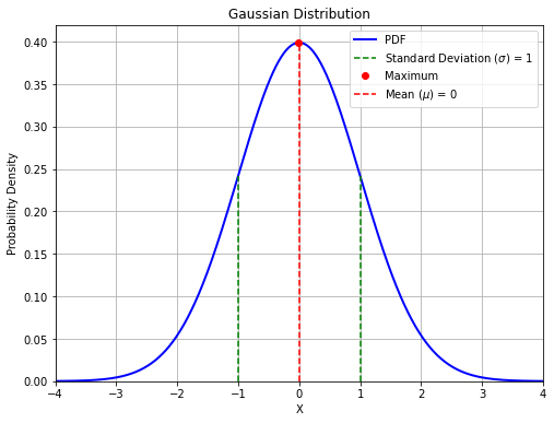
If we plot the PDF of a Normal distribution, we can find that it is easy to interpret the meaning of its parameters:

• The resulting curve has a maximum (highest probability) when \(x = \mu\)

• The curve is symmetric, with the inflection points at \(x = \mu \pm \sigma\)

• The example shows a normal distribution for \(\mu = 0\) and \(\sigma = 1\)

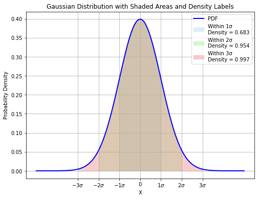
Another notable property of the Normal distribution is that:

• About \(68\%\) of the density is comprised in the interval \(\lbrack - \sigma,\sigma\rbrack\);

• About \(95\%\) of the density is comprised in the interval \(\lbrack - 2\sigma,2\sigma\rbrack\);

• Almost 100% of the density is comprised in the interval \(\lbrack - 3\sigma,3\sigma\rbrack\).

5.7.6.2. Multivariate Gaussian

The formulation of the Gaussian distribution generalizes to the multivariate case, i.e., the case in which \(X\) is n-dimensional.

In that case, the distribution is parametrized by a n-dimensional vector \(\mathbf{\mu}\) and a \(\mathbf{n}\mathbf{\times}\mathbf{n}\mathbf{\ }\)positive definite symmetric matrix \(\mathbf{\Sigma}\). The formulation of the multi-variate Gaussian is:

\[N\left( \mathbf{x;\mu,}\mathbf{\Sigma} \right) = \sqrt{\frac{1}{(2\pi)^{n}\det(\Sigma)}}e^{( - \frac{1}{2}\left( \mathbf{x} - \mathbf{\mu} \right)^{T}\Sigma^{- 1}\left( \mathbf{x} - \mathbf{\mu} \right))}\]

In the 2D case, \(\mathbf{\mu}\) is a 2D point representing the center of the Gaussian (the position of the mode), whereas the matrix \(\Sigma\) influences the “shape” of the Gaussian.

Examples of bivariate Gaussian distributions are shown below.

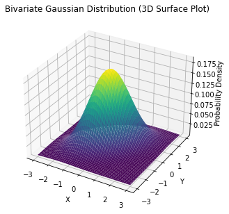
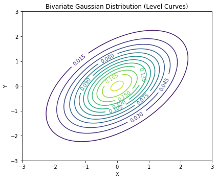
The two plots above are common representations for bivariate continuous distributions:

• The plot on the top shows a 3D representation of the PDF in which the X and Y axes are the values of the variables, while the third axis reports the probability density.

• Since it’s often hard to draw 3D graphs, we often use a contour plot to represent the 3D curves. In the 3D plot, curves of the same color represent points which have the same density in the 3D plot.

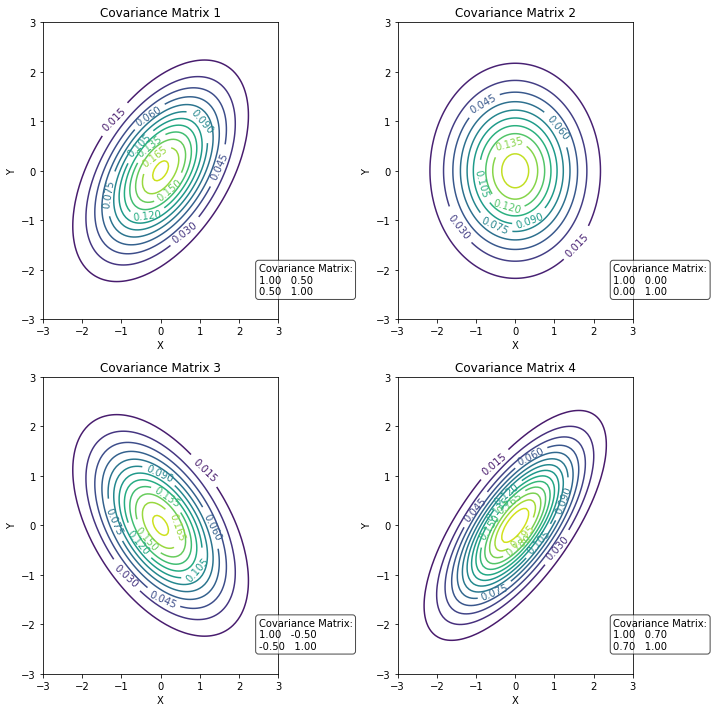
5.7.6.3. Effect of \(\Sigma\)

Similar to how variance affects the dispersion of a 1D Gaussian, the covariance matrix \(\Sigma\) affects the dispersion in both axes. As a result, changing the values of the matrix will affect the shape of the distribution. Let’s consider the general covariance matrix:

\[\begin{split} \Sigma = \begin{bmatrix} \sigma_x^2 & \sigma_{xy} \\ \sigma_{yx} & \sigma_y^2 \end{bmatrix} \end{split}\]

If the matrix is diagonal (\(\sigma_{xy}=\sigma_{yx}=0\)), then we have an isotropic Gaussian, meaning that it is symmetric along the two axes. Adding values different from zeros in the secondary diagonal will change the shape. Some examples are shown below:

5.7.6.4. Estimation of the Parameters of a Gaussian Distribution

We have noted that in many cases we can assume a random variable follows a Gaussian distribution. However, it is not yet clear how to choose the parameters of the Gaussian distribution.

Given some data (remember, data is values assumed by random variables!), we can obtain the parameters of the Gaussian distribution related to the data with a maximum likelihood estimation.

This consists in computing the mean and variance parameters using the following formula (in the univariate case):

• \(\mu = \frac{1}{n}\sum_{j}^{}x_{j}\)

• \(\sigma^{2} = \frac{1}{n}\sum_{j}^{}\left( x_{j} - \mu \right)^{2}\)

Where \(x_{j}\) represent the different data points.

In the multi-variate case, the computation of the multi-dimensional \(\mathbf{\mu}\) vector is similar:

• \(\mathbf{\mu} = \frac{1}{n}\sum_{j}^{}\mathbf{x}_{j}\)

• \(\Sigma\) is instead computed as the covariance matrix related to \(X\): \(\Sigma = Cov(\mathbf{X})\), i.e., \(\Sigma_{ij} = Cov\left( \mathbf{X}_{i},\mathbf{X}_{j} \right)\)

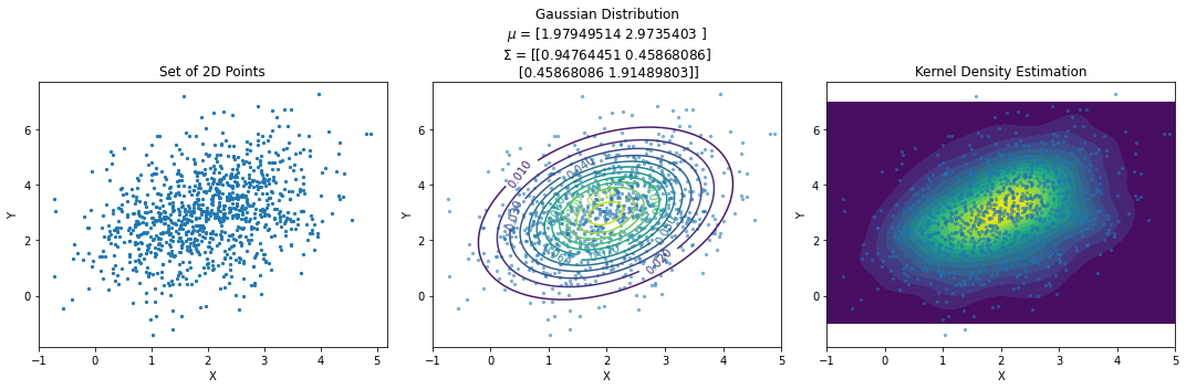
The diagram below shows an example in which we fit a Gaussian to a set of data and compare it with a 2D KDE of the data.

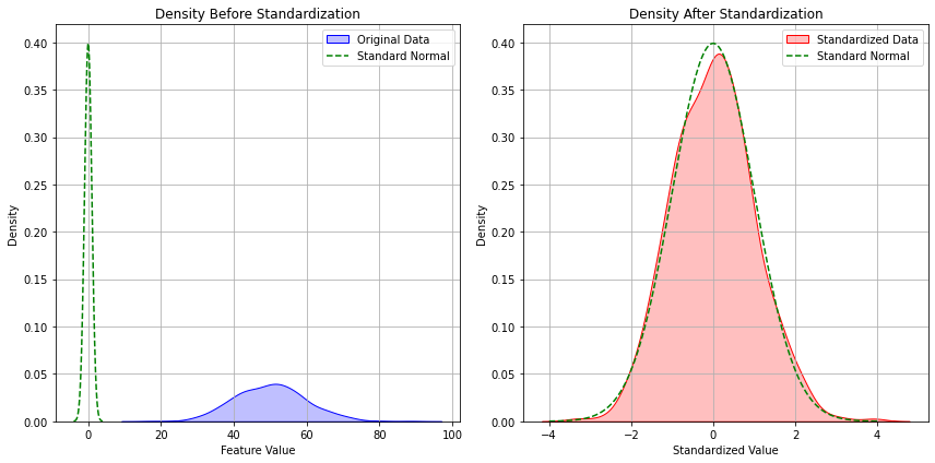
5.7.7. Standardization and Normal Distribution

We have seen that standardization gives rise to a new variable:

\[Z = \frac{X - \mu_X}{\sigma_X} = \frac{X-E[X]}{\sqrt{Var[X]}}\]

The plot below shows a data distribution before and after standardization.

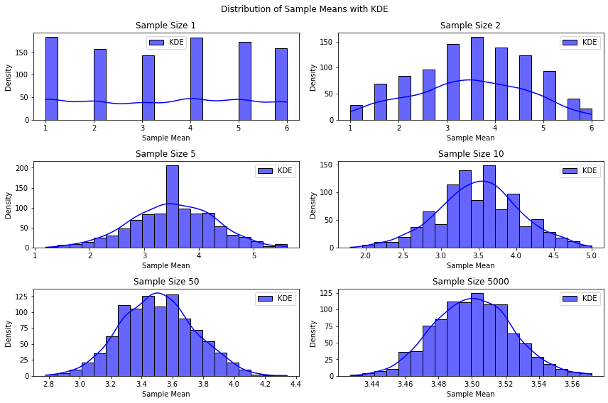
5.7.8. Central Limit Theorem

The Central Limit Theorem is a statistical principle that states that the distribution of the sum (or average) of a large number of independent, identically distributed (i.i.d.) random variables \(\{X_i\}_{i=1}^n\) approaches a normal distribution as \(n \to \infty\), regardless of the shape of the original population’s distribution.

While we will not see this theorem formally, it is a fundamental result which in some sense “justifies” the pervasive use of the Gaussian distribution in data analysis.

In the plot below, we plot the distributions of the average outcome of rolling a given number of dice. We can see each die as described by a different and independent random variable, hence the distribution will get close to Gaussian as we increase the number of dice.

5.8. Other Distributions (Optional)

5.8.1. Poisson Distribution

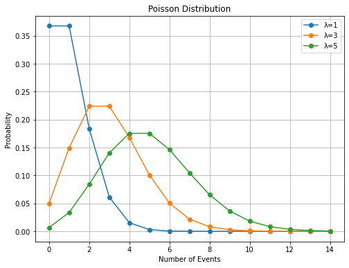
The Poisson distribution expresses the probability of a given number of events occurring in a fixed interval of time or space if they occur independently with a known rate. It is useful to model situations in which the number of events is very large and the probability of a given event happening is relatively small. The Poisson distribution is controlled by a parameter \(\lambda>0\) (the rate at which each event occurs) and defined as:

\[P(X=x) = \frac{\lambda^x}{x!}\exp(-\lambda)\]

with \(x=0,1,2,3,\ldots\) representing the number of events happening at the same time/space. The plot below shows the Poisson distribution for different choices of the \(\lambda\) parameter:

5.8.1.1. Example

During World War II Germans bombed the south of London many times. People started to believe that some areas were more targeted by the bombing and hence started moving from one part of a city to another in an attempt to avoid those areas.

After the end of the war, R. D. Charles showed that the bombings were actually random and independent. To do so, he divided the interested area in \(576\) squares of \(0.24 Km^2\). The number of total bombs was \(537\), hence less than one per square (a rare event). Assuming that the bombing was uniform and casual, the probability of a square being bombed would be:

\[\lambda = \frac{537}{576}\]

We can hence compute the expected probability that \(x\) squares were bombed as \(P(X=x)\), where \(P\) is a Poisson function with \(\lambda=\frac{537}{576}\). The expected number of areas being bombed \(x\) times will be: \(P(X=x)\times576\)

Comparing the expected numbers with the measured ones, we obtain the following table:

	Expected	Real
0	226.742723	229
1	211.390351	211
2	98.538731	93
3	30.622279	35
4	7.137224	8

Since the numbers are very close, we can imagine that the bombing was really random.

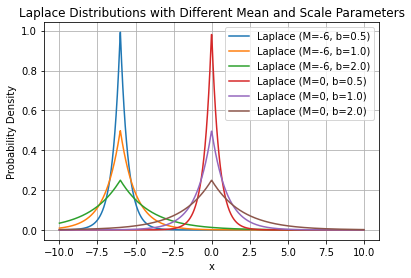
5.8.2. Laplacian Distribution

The Gaussian distribution assumes that the probability of an observation deviating from the mean decreases exponentially as the square of the deviation. For some types of data, this assumption is not accurate: in some cases, deviating from the mean is much more likely than prescribed by the Gaussian model. An alternative mathematical model, introduced by Laplace, posits that the probability of an observation deviating from the mean decreases exponentially with the absolute value of the deviation:

\[L(x, M, b) = \frac{1}{2b} e^{-\frac{|x - M|}{b}}\]

Where \(M\) represents the central/mean value of the distribution, and b is a scaling parameter known as diversity. It should be noted that due to the absolute value involved, this function is not differentiable at the mean value.

The best fit of this function to the data occurs when M is chosen as the median of the data, and b is chosen as the mean of the absolute differences between the data points and the median:

\[M=median(\{x_i\}_{i=1}^n)\]

\[b=\frac{\sum_{i=1}^n|x_i-M|}{n}\]

In this model, values far from the central value occur more frequently than they would in a Gaussian model. This phenomenon is referred to as fat tails in contrast to the Gaussian model, which is described as having thin tails.

Expectation and variance of \(X \sim L\) are:

\[E[X] = \lambda\]

\[Var(X) = \lambda\]

The following plot shows some examples of Laplacian distributions:

5.9. References

• Parts of chapter 1 of [1];

• Most of chapter 3 of [2];

• Parts of chapter 8 of [3].

[1] Bishop, Christopher M. Pattern recognition and machine learning. springer, 2006. https://www.microsoft.com/en-us/research/uploads/prod/2006/01/Bishop-Pattern-Recognition-and-Machine-Learning-2006.pdf

[2] Goodfellow, Ian, Yoshua Bengio, and Aaron Courville. Deep learning. MIT press, 2016. https://www.deeplearningbook.org/

[3] Heumann, Christian, and Michael Schomaker Shalabh. Introduction to statistics and data analysis. Springer International Publishing Switzerland, 2016.