Exploratory/Inferential Analysis on the Heart Disease Dataset

Contents

27. Exploratory/Inferential Analysis on the Heart Disease Dataset#

pip install ucimlrepo

Collecting ucimlrepo
  Downloading ucimlrepo-0.0.7-py3-none-any.whl.metadata (5.5 kB)
Requirement already satisfied: pandas>=1.0.0 in /usr/local/lib/python3.10/dist-packages (from ucimlrepo) (2.2.2)
Requirement already satisfied: certifi>=2020.12.5 in /usr/local/lib/python3.10/dist-packages (from ucimlrepo) (2024.8.30)
Requirement already satisfied: numpy>=1.22.4 in /usr/local/lib/python3.10/dist-packages (from pandas>=1.0.0->ucimlrepo) (1.26.4)
Requirement already satisfied: python-dateutil>=2.8.2 in /usr/local/lib/python3.10/dist-packages (from pandas>=1.0.0->ucimlrepo) (2.8.2)
Requirement already satisfied: pytz>=2020.1 in /usr/local/lib/python3.10/dist-packages (from pandas>=1.0.0->ucimlrepo) (2024.2)
Requirement already satisfied: tzdata>=2022.7 in /usr/local/lib/python3.10/dist-packages (from pandas>=1.0.0->ucimlrepo) (2024.2)
Requirement already satisfied: six>=1.5 in /usr/local/lib/python3.10/dist-packages (from python-dateutil>=2.8.2->pandas>=1.0.0->ucimlrepo) (1.16.0)
Downloading ucimlrepo-0.0.7-py3-none-any.whl (8.0 kB)
Installing collected packages: ucimlrepo
Successfully installed ucimlrepo-0.0.7

Carichiamo i dati dal repository di UCI ML

from ucimlrepo import fetch_ucirepo

# fetch dataset
heart_disease = fetch_ucirepo(id=45)

# data (as pandas dataframes)
X = heart_disease.data.features
y = heart_disease.data.targets

data = X.join(y)
data

	age	sex	cp	trestbps	chol	fbs	restecg	thalach	exang	oldpeak	slope	ca	thal	num
0	63	1	1	145	233	1	2	150	0	2.3	3	0.0	6.0	0
1	67	1	4	160	286	0	2	108	1	1.5	2	3.0	3.0	2
2	67	1	4	120	229	0	2	129	1	2.6	2	2.0	7.0	1
3	37	1	3	130	250	0	0	187	0	3.5	3	0.0	3.0	0
4	41	0	2	130	204	0	2	172	0	1.4	1	0.0	3.0	0
...	...	...	...	...	...	...	...	...	...	...	...	...	...	...
298	45	1	1	110	264	0	0	132	0	1.2	2	0.0	7.0	1
299	68	1	4	144	193	1	0	141	0	3.4	2	2.0	7.0	2
300	57	1	4	130	131	0	0	115	1	1.2	2	1.0	7.0	3
301	57	0	2	130	236	0	2	174	0	0.0	2	1.0	3.0	1
302	38	1	3	138	175	0	0	173	0	0.0	1	NaN	3.0	0

303 rows × 14 columns

#import pandas as pd
#pd.read_csv('heart.csv')

data.info()

<class 'pandas.core.frame.DataFrame'>
RangeIndex: 303 entries, 0 to 302
Data columns (total 14 columns):
 #   Column    Non-Null Count  Dtype  
---  ------    --------------  -----  
 0   age       303 non-null    int64  
 1   sex       303 non-null    int64  
 2   cp        303 non-null    int64  
 3   trestbps  303 non-null    int64  
 4   chol      303 non-null    int64  
 5   fbs       303 non-null    int64  
 6   restecg   303 non-null    int64  
 7   thalach   303 non-null    int64  
 8   exang     303 non-null    int64  
 9   oldpeak   303 non-null    float64
 10  slope     303 non-null    int64  
 11  ca        299 non-null    float64
 12  thal      301 non-null    float64
 13  num       303 non-null    int64  
dtypes: float64(3), int64(11)
memory usage: 33.3 KB

for column in data.columns:
  x = data[column].isna().sum()
  print("Number of NaN in column", column, "is", x)

Number of NaN in column age is 0
Number of NaN in column sex is 0
Number of NaN in column cp is 0
Number of NaN in column trestbps is 0
Number of NaN in column chol is 0
Number of NaN in column fbs is 0
Number of NaN in column restecg is 0
Number of NaN in column thalach is 0
Number of NaN in column exang is 0
Number of NaN in column oldpeak is 0
Number of NaN in column slope is 0
Number of NaN in column ca is 4
Number of NaN in column thal is 2
Number of NaN in column num is 0

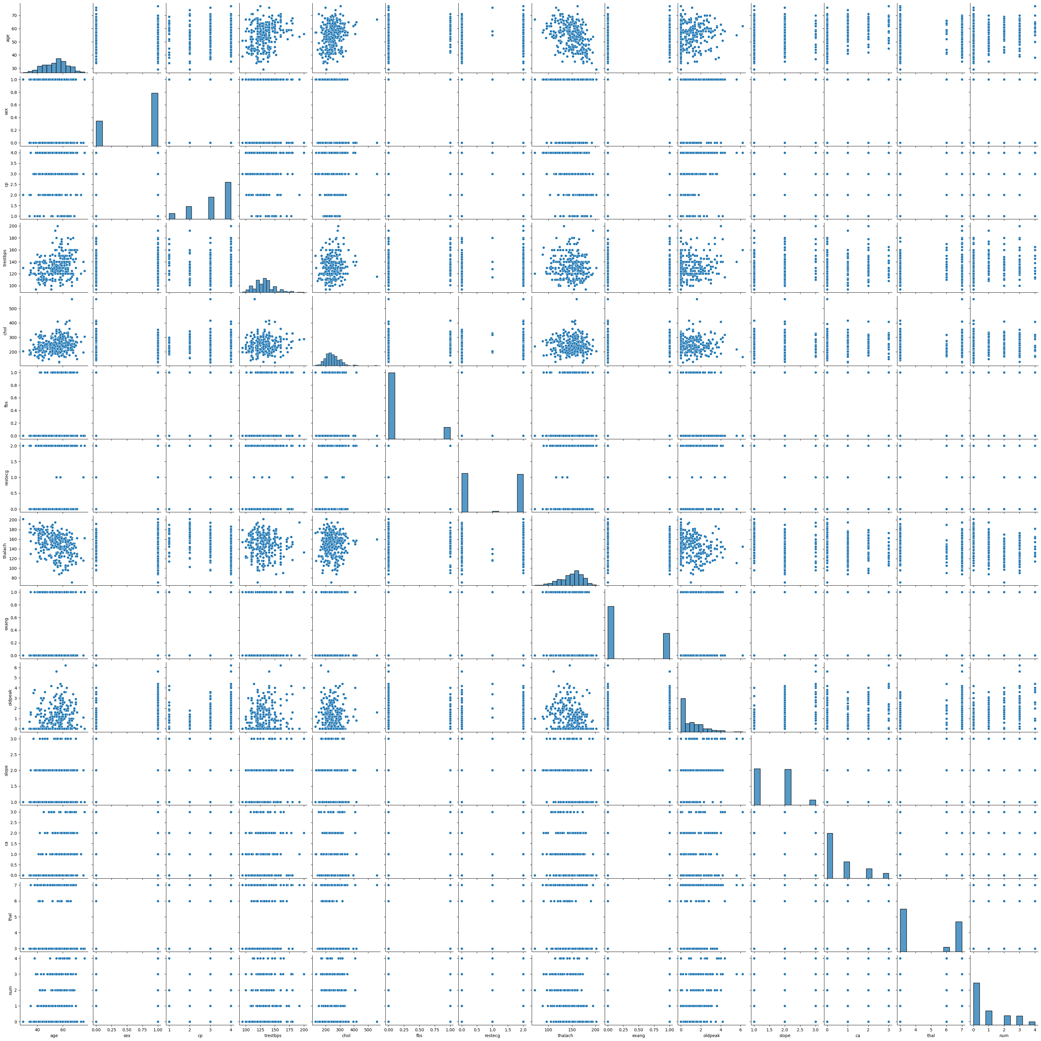
import seaborn as sns

sns.pairplot(data)

<seaborn.axisgrid.PairGrid at 0x7b5cf0507370>

../_images/b483707d2e4b9da2a2a60e4c22cfe851383dbb8ab76819ae0963e2671d2fa7ed.png

data['num'].unique()

array([0, 2, 1, 3, 4])

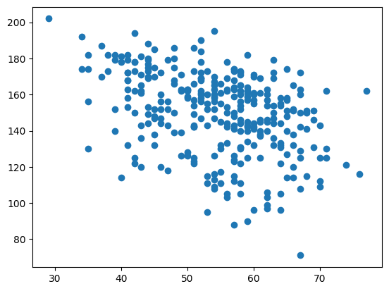
27.1. Does age affect maximum heart rate?#

from matplotlib import pyplot as plt
plt.scatter(data['age'], data['thalach'])
plt.show()

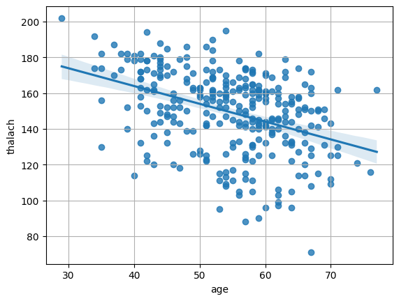
../_images/4dd92440c0b9af67adafa6fca458b6128a9bdd03db023901f5236122b5d4cea1.png

from scipy.stats import pearsonr

pearsonr(data['age'], data['thalach'])

PearsonRResult(statistic=-0.3938058059868209, pvalue=1.1092756352878365e-12)

sns.regplot(data, x='age', y='thalach')
plt.grid()

../_images/26edf8ec9ab9c6cebed7f3bd30f3f1ea7e5d1e346313f0f6b8dbe803d042f083.png

from statsmodels.formula.api import ols

ols("thalach ~ age", data).fit().summary()

OLS Regression Results
Dep. Variable:	thalach	R-squared:	0.155
Model:	OLS	Adj. R-squared:	0.152
Method:	Least Squares	F-statistic:	55.25
Date:	Thu, 21 Nov 2024	Prob (F-statistic):	1.11e-12
Time:	16:54:49	Log-Likelihood:	-1352.3
No. Observations:	303	AIC:	2709.
Df Residuals:	301	BIC:	2716.
Df Model:	1
Covariance Type:	nonrobust

	coef	std err	t	P>\|t\|	[0.025	0.975]
Intercept	203.8634	7.399	27.553	0.000	189.303	218.424
age	-0.9966	0.134	-7.433	0.000	-1.261	-0.733

Omnibus:	19.198	Durbin-Watson:	1.744
Prob(Omnibus):	0.000	Jarque-Bera (JB):	21.705
Skew:	-0.654	Prob(JB):	1.94e-05
Kurtosis:	2.922	Cond. No.	338.

Notes:
[1] Standard Errors assume that the covariance matrix of the errors is correctly specified.

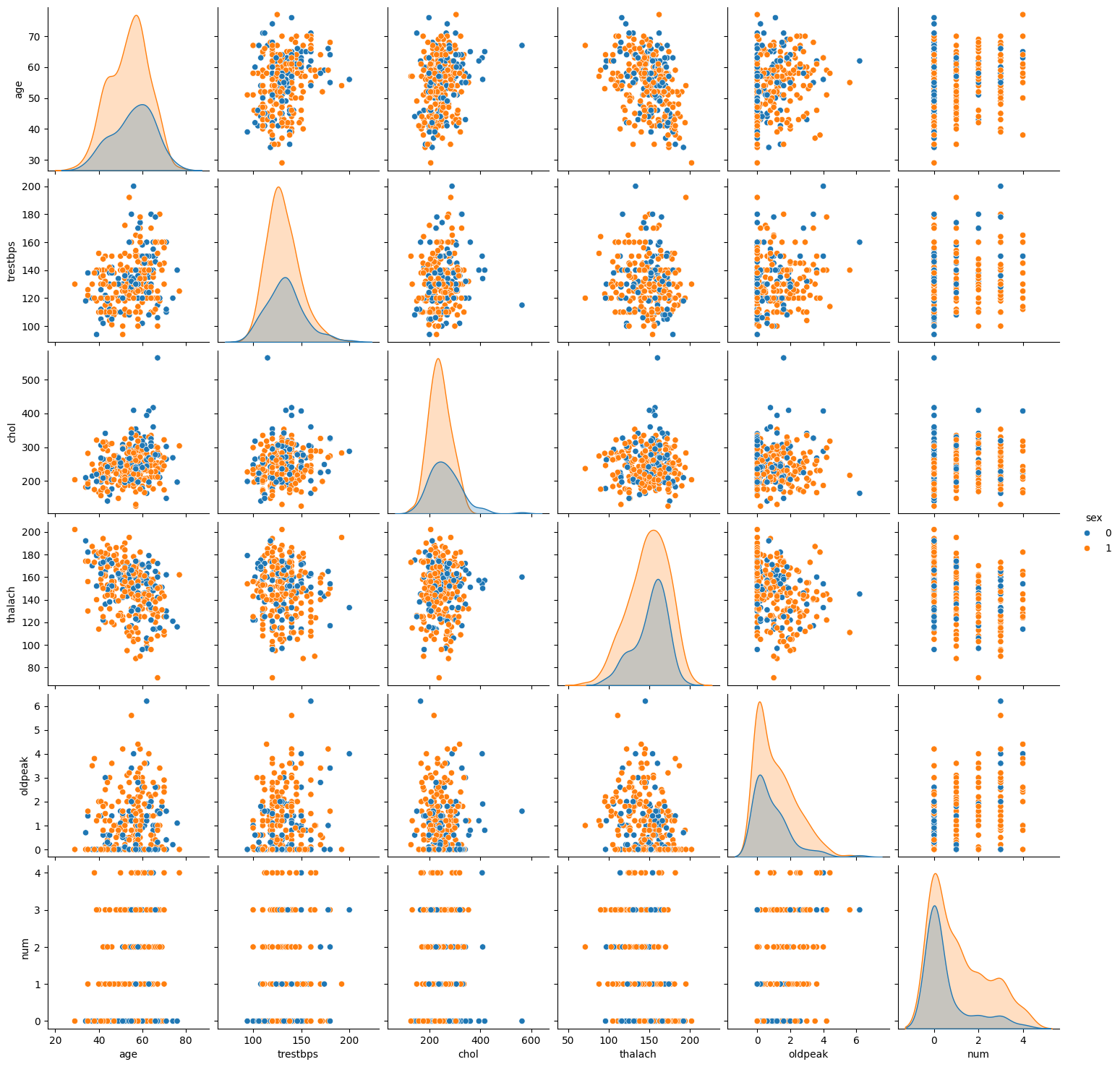
import seaborn as sns

sns.pairplot(data.drop(['cp','fbs','restecg','exang','slope','ca','thal'], axis=1), hue='sex')

<seaborn.axisgrid.PairGrid at 0x7b5cd56825c0>

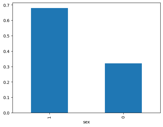
../_images/d7f25bf799540a53aa1f47df342119bae3d2ebc3a4d9bd6ef474adc9cc84ed4c.png

data['sex'].value_counts().plot.bar()

<Axes: xlabel='sex'>

../_images/7a479e0b59f6fb4d55adfe68b9bbfe52e24f1bd38e61fc3a5db41621d5bd6cf9.png

data['sex'].value_counts(normalize=True).plot.bar()

<Axes: xlabel='sex'>

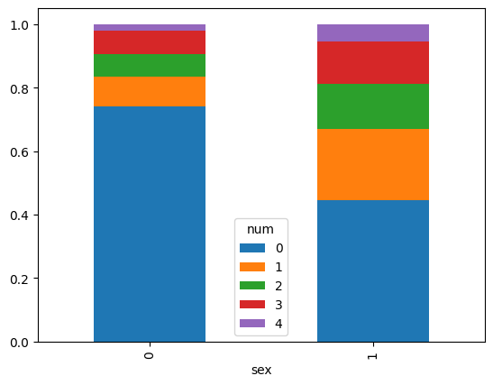
../_images/34f75ac7eebed82909390d9414d16a79abb4e917c6ea1974a62dd4e0e7ca793f.png

pd.crosstab(data['sex'], data['num'],normalize='index').plot.bar(stacked=True)

<Axes: xlabel='sex'>

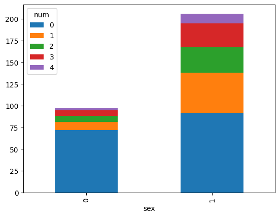
../_images/a197f19ea2dd389b3b76d9be5ed3801c68dd7fef6c5e392d7b3b07d6ebc4045e.png

pd.crosstab(data['sex'], data['num']).plot.bar(stacked=True)

<Axes: xlabel='sex'>

../_images/5f0bf41f8b7db67bd3563317675ea828e528651570abeb3e8c629613dee0e060.png

from scipy.stats import chi2_contingency
from scipy.stats.contingency import association

# Perform the Chi-Square Test for Independence
contingency_table = pd.crosstab(data['sex'], data['num'])
chi2, p, _, exp_freq = chi2_contingency(contingency_table)

# Set the significance level (alpha)
alpha = 0.05

# Print the results
print("Chi-Square Statistic:", chi2)
print("p-value:", p)

print("Cramer's V:", association(contingency_table))

# Interpret the results
if p < alpha:
    print("\nThere is a significant association between 'Sex' and 'survived'.")
else:
    print("\nThere is no significant association between 'Sex' and 'survived'.")

Chi-Square Statistic: 23.425407307562654
p-value: 0.00010410590365461076
Cramer's V: 0.27804959139060786

There is a significant association between 'Sex' and 'survived'.

data_binary = data.copy()
data_binary['num'] = data_binary['num'].apply(lambda x: 1 if x >= 1 else 0)
crosstab_binary = pd.crosstab(data_binary['sex'], data_binary['num'])
crosstab_binary

num	0	1
sex
0	72	25
1	92	114

from scipy.stats.contingency import relative_risk
relative_risk(crosstab_binary[1][1], crosstab_binary[1].sum(), crosstab_binary[0][1], crosstab_binary[0].sum())
#relative_risk(contingency['Exposed']['Diseased'],contingency['Exposed'].sum(),contingency['Non Exposed']['Diseased'], contingency['Non Exposed'].sum())

RelativeRiskResult(relative_risk=1.4619956208945886, exposed_cases=114, exposed_total=139, control_cases=92, control_total=164)

# prompt: can you invert the rows of crosstab_binary

crosstab_binary_inverted = crosstab_binary.iloc[::-1]
crosstab_binary_inverted = crosstab_binary_inverted[[1,0]]
crosstab_binary_inverted

num	1	0
sex
1	114	92
0	25	72

from scipy.stats.contingency import odds_ratio

odds_ratio(crosstab_binary_inverted)

OddsRatioResult(statistic=3.55354424429681)

27.2. Logistic regression analysis on binarized data#

from statsmodels.formula.api import logit
logit("num ~ sex", data_binary).fit().summary()

Optimization terminated successfully.
         Current function value: 0.650054
         Iterations 5

Logit Regression Results
Dep. Variable:	num	No. Observations:	303
Model:	Logit	Df Residuals:	301
Method:	MLE	Df Model:	1
Date:	Thu, 21 Nov 2024	Pseudo R-squ.:	0.05754
Time:	17:36:26	Log-Likelihood:	-196.97
converged:	True	LL-Null:	-208.99
Covariance Type:	nonrobust	LLR p-value:	9.390e-07

	coef	std err	z	P>\|z\|	[0.025	0.975]
Intercept	-1.0578	0.232	-4.557	0.000	-1.513	-0.603
sex	1.2722	0.271	4.692	0.000	0.741	1.804

import numpy as np
odds = np.exp(-1.0578)
p = odds/(1+odds)
p

0.2577301019775979

np.exp(1.2722)

3.568695061578707

odds_m = odds*np.exp(1.2722)
odds_m/(1+odds_m)

0.5533956185614641

27.3. Multinomial Logistic Regression Analysis#

from statsmodels.formula.api import mnlogit
mnlogit("num ~ sex", data).fit().summary()

Optimization terminated successfully.
         Current function value: 1.239318
         Iterations 7

MNLogit Regression Results
Dep. Variable:	num	No. Observations:	303
Model:	MNLogit	Df Residuals:	295
Method:	MLE	Df Model:	4
Date:	Thu, 21 Nov 2024	Pseudo R-squ.:	0.03141
Time:	17:46:39	Log-Likelihood:	-375.51
converged:	True	LL-Null:	-387.69
Covariance Type:	nonrobust	LLR p-value:	6.775e-05

num=1	coef	std err	z	P>\|z\|	[0.025	0.975]
Intercept	-2.0794	0.354	-5.882	0.000	-2.772	-1.386
sex	1.3863	0.397	3.492	0.000	0.608	2.164
num=2	coef	std err	z	P>\|z\|	[0.025	0.975]
Intercept	-2.3308	0.396	-5.887	0.000	-3.107	-1.555
sex	1.1763	0.450	2.617	0.009	0.295	2.057
num=3	coef	std err	z	P>\|z\|	[0.025	0.975]
Intercept	-2.3308	0.396	-5.887	0.000	-3.107	-1.555
sex	1.1412	0.451	2.531	0.011	0.257	2.025
num=4	coef	std err	z	P>\|z\|	[0.025	0.975]
Intercept	-3.5835	0.717	-4.999	0.000	-4.989	-2.178
sex	1.4596	0.785	1.860	0.063	-0.078	2.998

odds1=np.exp(-2.0794)

odds2=np.exp(-2.0794)*np.exp(1.3863)

p1 = odds1/(1+odds1)
p2 = odds2/(1+odds2)

print(p1, p2)

0.11111521405935315 0.3333438179846534