import pandas as pd
data = pd.read_csv('BankChurners.csv').set_index('CLIENTNUM')
data

	Attrition_Flag	Customer_Age	Gender	Dependent_count	Education_Level	Marital_Status	Income_Category	Card_Category	Months_on_book	Total_Relationship_Count	...	Credit_Limit	Total_Revolving_Bal	Avg_Open_To_Buy	Total_Amt_Chng_Q4_Q1	Total_Trans_Amt	Total_Trans_Ct	Total_Ct_Chng_Q4_Q1	Avg_Utilization_Ratio	Naive_Bayes_Classifier_Attrition_Flag_Card_Category_Contacts_Count_12_mon_Dependent_count_Education_Level_Months_Inactive_12_mon_1	Naive_Bayes_Classifier_Attrition_Flag_Card_Category_Contacts_Count_12_mon_Dependent_count_Education_Level_Months_Inactive_12_mon_2
CLIENTNUM
768805383	Existing Customer	45	M	3	High School	Married	$60K - $80K	Blue	39	5	...	12691.0	777	11914.0	1.335	1144	42	1.625	0.061	0.000093	0.999910
818770008	Existing Customer	49	F	5	Graduate	Single	Less than $40K	Blue	44	6	...	8256.0	864	7392.0	1.541	1291	33	3.714	0.105	0.000057	0.999940
713982108	Existing Customer	51	M	3	Graduate	Married	$80K - $120K	Blue	36	4	...	3418.0	0	3418.0	2.594	1887	20	2.333	0.000	0.000021	0.999980
769911858	Existing Customer	40	F	4	High School	Unknown	Less than $40K	Blue	34	3	...	3313.0	2517	796.0	1.405	1171	20	2.333	0.760	0.000134	0.999870
709106358	Existing Customer	40	M	3	Uneducated	Married	$60K - $80K	Blue	21	5	...	4716.0	0	4716.0	2.175	816	28	2.500	0.000	0.000022	0.999980
...	...	...	...	...	...	...	...	...	...	...	...	...	...	...	...	...	...	...	...	...	...
772366833	Existing Customer	50	M	2	Graduate	Single	$40K - $60K	Blue	40	3	...	4003.0	1851	2152.0	0.703	15476	117	0.857	0.462	0.000191	0.999810
710638233	Attrited Customer	41	M	2	Unknown	Divorced	$40K - $60K	Blue	25	4	...	4277.0	2186	2091.0	0.804	8764	69	0.683	0.511	0.995270	0.004729
716506083	Attrited Customer	44	F	1	High School	Married	Less than $40K	Blue	36	5	...	5409.0	0	5409.0	0.819	10291	60	0.818	0.000	0.997880	0.002118
717406983	Attrited Customer	30	M	2	Graduate	Unknown	$40K - $60K	Blue	36	4	...	5281.0	0	5281.0	0.535	8395	62	0.722	0.000	0.996710	0.003294
714337233	Attrited Customer	43	F	2	Graduate	Married	Less than $40K	Silver	25	6	...	10388.0	1961	8427.0	0.703	10294	61	0.649	0.189	0.996620	0.003377

10127 rows × 22 columns

data.info()

<class 'pandas.core.frame.DataFrame'>
Index: 10127 entries, 768805383 to 714337233
Data columns (total 22 columns):
 #   Column                                                                                                                              Non-Null Count  Dtype  
---  ------                                                                                                                              --------------  -----  
 0   Attrition_Flag                                                                                                                      10127 non-null  object 
 1   Customer_Age                                                                                                                        10127 non-null  int64  
 2   Gender                                                                                                                              10127 non-null  object 
 3   Dependent_count                                                                                                                     10127 non-null  int64  
 4   Education_Level                                                                                                                     10127 non-null  object 
 5   Marital_Status                                                                                                                      10127 non-null  object 
 6   Income_Category                                                                                                                     10127 non-null  object 
 7   Card_Category                                                                                                                       10127 non-null  object 
 8   Months_on_book                                                                                                                      10127 non-null  int64  
 9   Total_Relationship_Count                                                                                                            10127 non-null  int64  
 10  Months_Inactive_12_mon                                                                                                              10127 non-null  int64  
 11  Contacts_Count_12_mon                                                                                                               10127 non-null  int64  
 12  Credit_Limit                                                                                                                        10127 non-null  float64
 13  Total_Revolving_Bal                                                                                                                 10127 non-null  int64  
 14  Avg_Open_To_Buy                                                                                                                     10127 non-null  float64
 15  Total_Amt_Chng_Q4_Q1                                                                                                                10127 non-null  float64
 16  Total_Trans_Amt                                                                                                                     10127 non-null  int64  
 17  Total_Trans_Ct                                                                                                                      10127 non-null  int64  
 18  Total_Ct_Chng_Q4_Q1                                                                                                                 10127 non-null  float64
 19  Avg_Utilization_Ratio                                                                                                               10127 non-null  float64
 20  Naive_Bayes_Classifier_Attrition_Flag_Card_Category_Contacts_Count_12_mon_Dependent_count_Education_Level_Months_Inactive_12_mon_1  10127 non-null  float64
 21  Naive_Bayes_Classifier_Attrition_Flag_Card_Category_Contacts_Count_12_mon_Dependent_count_Education_Level_Months_Inactive_12_mon_2  10127 non-null  float64
dtypes: float64(7), int64(9), object(6)
memory usage: 1.8+ MB

data['Attrition_Flag'].unique()

array(['Existing Customer', 'Attrited Customer'], dtype=object)

data['Education_Level'].unique()

array(['High School', 'Graduate', 'Uneducated', 'Unknown', 'College',
       'Post-Graduate', 'Doctorate'], dtype=object)

data['Marital_Status'].unique()

array(['Married', 'Single', 'Unknown', 'Divorced'], dtype=object)

data['Income_Category'].unique()

array(['$60K - $80K', 'Less than $40K', '$80K - $120K', '$40K - $60K',
       '$120K +', 'Unknown'], dtype=object)

data['Card_Category'].unique()

array(['Blue', 'Gold', 'Silver', 'Platinum'], dtype=object)

33. Clustering

data2 = data.copy()
data2 = data2.drop(['Attrition_Flag','Naive_Bayes_Classifier_Attrition_Flag_Card_Category_Contacts_Count_12_mon_Dependent_count_Education_Level_Months_Inactive_12_mon_1','Naive_Bayes_Classifier_Attrition_Flag_Card_Category_Contacts_Count_12_mon_Dependent_count_Education_Level_Months_Inactive_12_mon_2'], axis=1)

data2.head()

	Customer_Age	Gender	Dependent_count	Education_Level	Marital_Status	Income_Category	Card_Category	Months_on_book	Total_Relationship_Count	Months_Inactive_12_mon	Contacts_Count_12_mon	Credit_Limit	Total_Revolving_Bal	Avg_Open_To_Buy	Total_Amt_Chng_Q4_Q1	Total_Trans_Amt	Total_Trans_Ct	Total_Ct_Chng_Q4_Q1	Avg_Utilization_Ratio
CLIENTNUM
768805383	45	M	3	High School	Married	$60K - $80K	Blue	39	5	1	3	12691.0	777	11914.0	1.335	1144	42	1.625	0.061
818770008	49	F	5	Graduate	Single	Less than $40K	Blue	44	6	1	2	8256.0	864	7392.0	1.541	1291	33	3.714	0.105
713982108	51	M	3	Graduate	Married	$80K - $120K	Blue	36	4	1	0	3418.0	0	3418.0	2.594	1887	20	2.333	0.000
769911858	40	F	4	High School	Unknown	Less than $40K	Blue	34	3	4	1	3313.0	2517	796.0	1.405	1171	20	2.333	0.760
709106358	40	M	3	Uneducated	Married	$60K - $80K	Blue	21	5	1	0	4716.0	0	4716.0	2.175	816	28	2.500	0.000

data2 = pd.get_dummies(data2)

from sklearn.cluster import KMeans
import numpy as np

kmeans = KMeans(n_clusters=5, random_state = 42)

kmeans.fit(data2)

KMeans(n_clusters=5, random_state=42)

In a Jupyter environment, please rerun this cell to show the HTML representation or trust the notebook.
On GitHub, the HTML representation is unable to render, please try loading this page with nbviewer.org.

pred = kmeans.predict(data2)
pred

array([2, 3, 0, ..., 3, 3, 3], dtype=int32)

# prompt: fai fit di un kmeans con 5 cluster su data2 usando uno standard scaler senza usare le pipeline di sklearn

from sklearn.preprocessing import StandardScaler

# Create a StandardScaler object
scaler = StandardScaler()

# Fit the scaler to your data
scaler.fit(data2)

# Transform the data using the fitted scaler
scaled_data = scaler.transform(data2)

# Now, fit the KMeans model on the scaled data
kmeans = KMeans(n_clusters=5, random_state=42, n_init = 'auto')
kmeans.fit(scaled_data)

# Predict cluster labels for your data
pred = kmeans.predict(scaled_data)

# Print or use the predictions as needed
pred

# prompt: fai fit di un kmeans con 5 cluster su data2 usando uno standard scaler e le pipeline di scikit-learn

from sklearn.pipeline import Pipeline
from sklearn.preprocessing import StandardScaler

pipeline = Pipeline([
    ('scaler', StandardScaler()),
    ('kmeans', KMeans(n_clusters=5, n_init = 'auto', random_state=42))
])

pipeline.fit(data2)
pred = pipeline.predict(data2)
pred

array([4, 1, 4, ..., 0, 4, 3], dtype=int32)

pipeline

Pipeline(steps=[('scaler', StandardScaler()),
                ('kmeans', KMeans(n_clusters=5, random_state=42))])

In a Jupyter environment, please rerun this cell to show the HTML representation or trust the notebook.
On GitHub, the HTML representation is unable to render, please try loading this page with nbviewer.org.

pipeline.named_steps['kmeans']

KMeans(n_clusters=5, random_state=42)

In a Jupyter environment, please rerun this cell to show the HTML representation or trust the notebook.
On GitHub, the HTML representation is unable to render, please try loading this page with nbviewer.org.

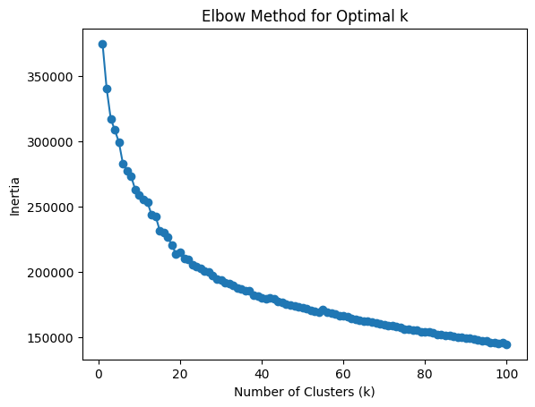
# prompt: trova il miglior K con metodo elbow

import matplotlib.pyplot as plt

# Calculate inertia for different values of k
inertia = []
k_values = range(1, 101)  # Test k values from 1 to 10

for k in k_values:
    pipeline = Pipeline([
        ('scaler', StandardScaler()),
        ('kmeans', KMeans(n_clusters=k, n_init='auto', random_state=42))
    ])
    pipeline.fit(data2)
    inertia.append(pipeline.named_steps['kmeans'].inertia_)

# Plot the elbow method graph
plt.plot(k_values, inertia, marker='o')
plt.xlabel('Number of Clusters (k)')
plt.ylabel('Inertia')
plt.title('Elbow Method for Optimal k')
plt.show()

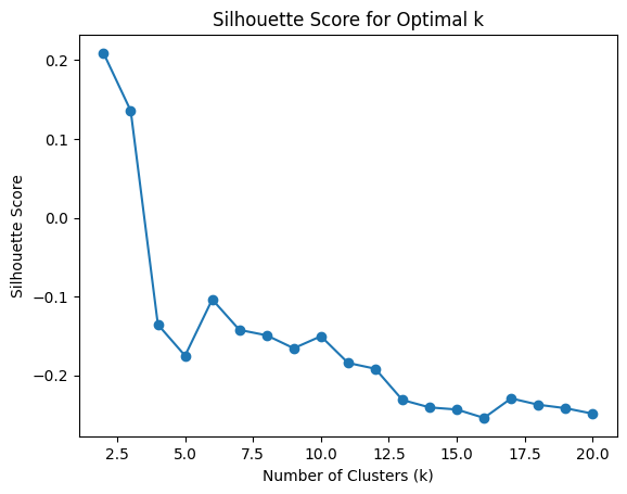
# prompt: trova il miglior k con silhoutte

from sklearn.metrics import silhouette_score
from sklearn.metrics import pairwise_distances

# Calculate silhouette scores for different values of k
silhouette_scores = []
k_values = range(2, 21)  # Test k values from 2 to 100 (Silhouette score is not defined for k=1)

pwd = pairwise_distances(data2)

for k in k_values:
    pipeline = Pipeline([
        ('scaler', StandardScaler()),
        ('kmeans', KMeans(n_clusters=k, n_init='auto', random_state=42))
    ])
    pipeline.fit(data2)
    labels = pipeline.predict(data2)
    silhouette_avg = silhouette_score(pwd, labels, metric='precomputed')
    silhouette_scores.append(silhouette_avg)

# Find the best k based on the highest silhouette score
best_k = k_values[np.argmax(silhouette_scores)]
print(f"Best k based on Silhouette score: {best_k}")

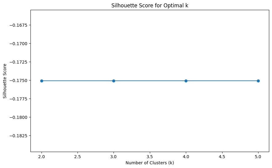
# Plot the silhouette scores
plt.plot(k_values, silhouette_scores, marker='o')
plt.xlabel('Number of Clusters (k)')
plt.ylabel('Silhouette Score')
plt.title('Silhouette Score for Optimal k')
plt.show()

Best k based on Silhouette score: 2

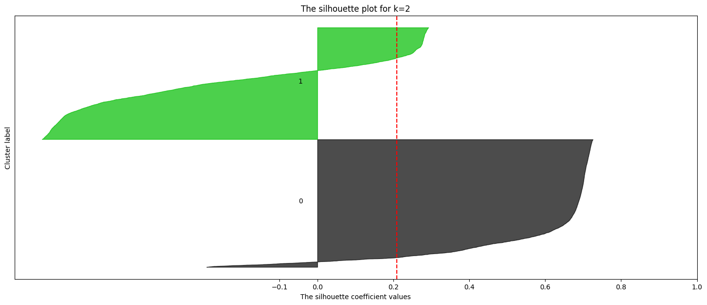
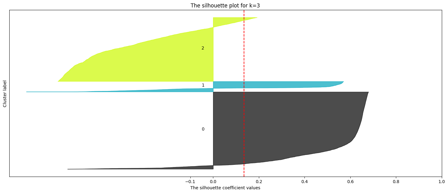
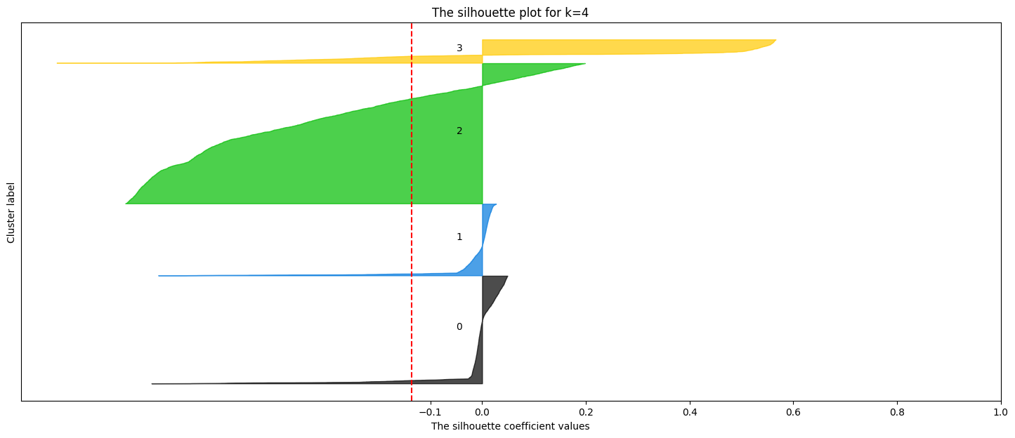
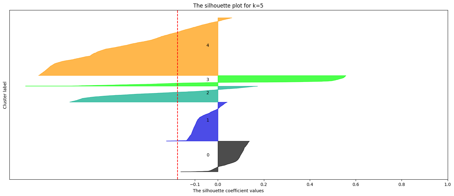
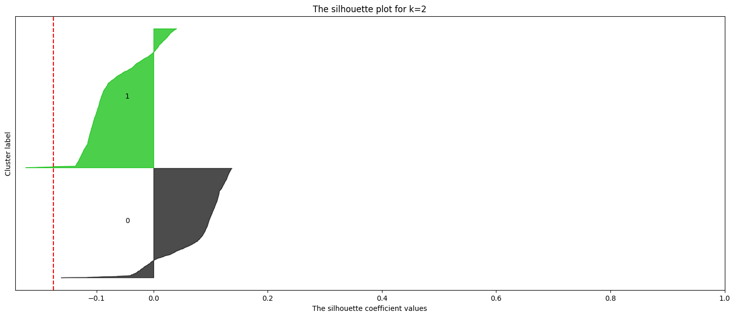
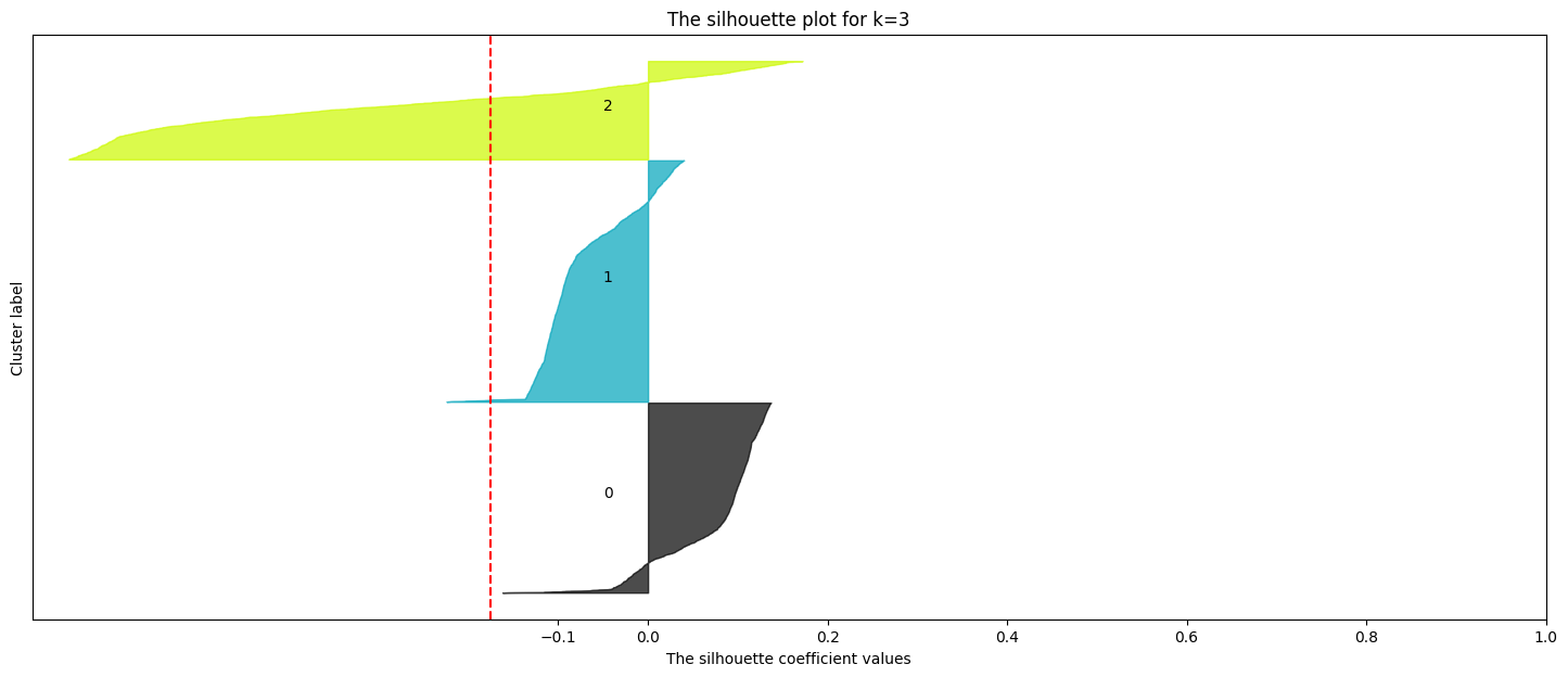
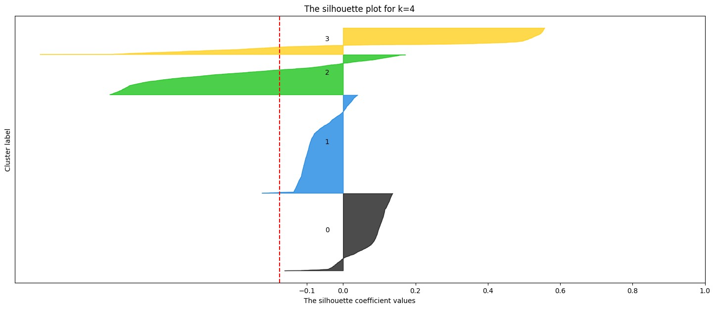
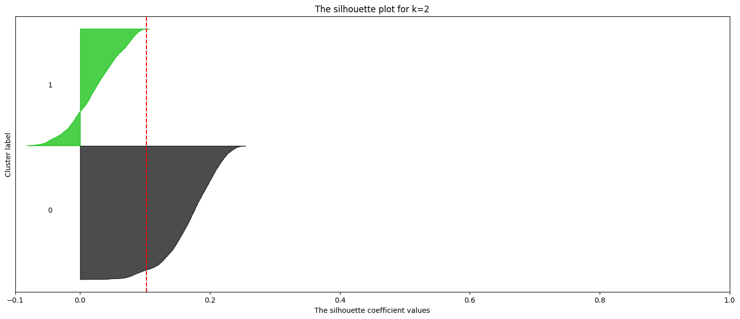
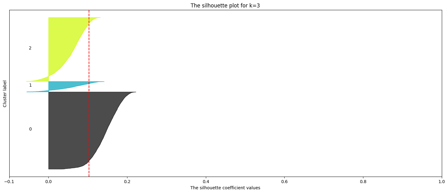
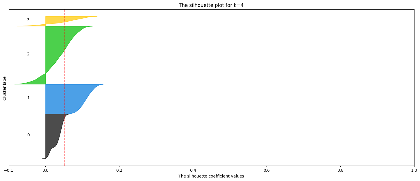
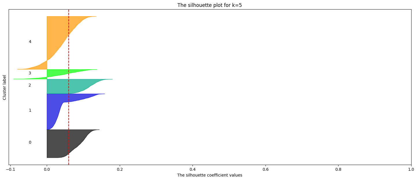
# prompt: effettua la silhouette analysis per k=range(1,6)
import matplotlib.cm as cm
import matplotlib.pyplot as plt
import numpy as np

from sklearn.cluster import KMeans
from sklearn.datasets import make_blobs
from sklearn.metrics import silhouette_samples, silhouette_score

# Calculate silhouette scores for different values of k
silhouette_scores = []
k_values = range(2, 6)  # Test k values from 2 to 5 (Silhouette score is not defined for k=1)

for k in k_values:
    pipeline = Pipeline([
        ('scaler', StandardScaler()),
        ('kmeans', KMeans(n_clusters=k, n_init='auto', random_state=42))
    ])
    pipeline.fit(data2)
    cluster_labels = pipeline.predict(data2)
    silhouette_avg = silhouette_score(data2, cluster_labels) # Use data2 directly here
    silhouette_scores.append(silhouette_avg)
    sample_silhouette_values = silhouette_samples(data2, cluster_labels)

    fig, (ax1) = plt.subplots(1, 1)
    fig.set_size_inches(18, 7)


    # The 1st subplot is the silhouette plot
    # The silhouette coefficient can range from -1, 1 but in this example all
    # lie within [-0.1, 1]
    #ax1.set_xlim([-0.1, 1])
    # The (n_clusters+1)*10 is for inserting blank space between silhouette
    # plots of individual clusters, to demarcate them clearly.
    #ax1.set_ylim([0, len(data2) + (k + 1) * 10])

    y_lower = 10
    for i in range(k):
        # Aggregate the silhouette scores for samples belonging to
        # cluster i, and sort them
        ith_cluster_silhouette_values = sample_silhouette_values[cluster_labels == i]

        ith_cluster_silhouette_values.sort()

        size_cluster_i = ith_cluster_silhouette_values.shape[0]
        y_upper = y_lower + size_cluster_i

        color = cm.nipy_spectral(float(i) / k)
        ax1.fill_betweenx(
            np.arange(y_lower, y_upper),
            0,
            ith_cluster_silhouette_values,
            facecolor=color,
            edgecolor=color,
            alpha=0.7,
        )

        # Label the silhouette plots with their cluster numbers at the middle
        ax1.text(-0.05, y_lower + 0.5 * size_cluster_i, str(i))

        # Compute the new y_lower for next plot
        y_lower = y_upper + 10  # 10 for the 0 samples

    ax1.set_title(f"The silhouette plot for k={k}")
    ax1.set_xlabel("The silhouette coefficient values")
    ax1.set_ylabel("Cluster label")

    # The vertical line for average silhouette score of all the values
    ax1.axvline(x=silhouette_avg, color="red", linestyle="--")

    ax1.set_yticks([])  # Clear the yaxis labels / ticks
    ax1.set_xticks([-0.1, 0, 0.2, 0.4, 0.6, 0.8, 1])

# Find the best k based on the highest silhouette score
best_k = k_values[np.argmax(silhouette_scores)]
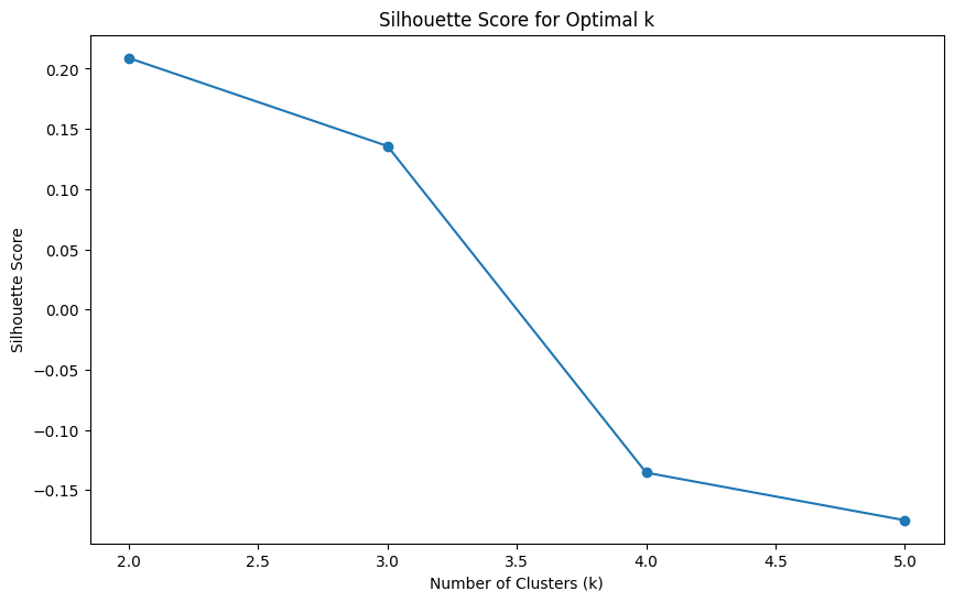
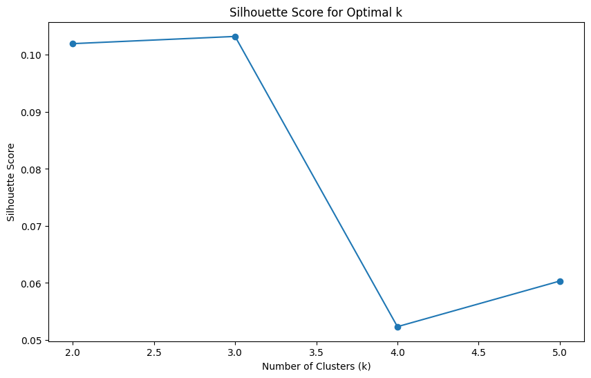
print(f"Best k based on Silhouette score: {best_k}")

# Plot the silhouette scores
plt.figure(figsize=(10, 6))
plt.plot(k_values, silhouette_scores, marker='o')
plt.xlabel('Number of Clusters (k)')
plt.ylabel('Silhouette Score')
plt.title('Silhouette Score for Optimal k')
plt.show()

Best k based on Silhouette score: 2

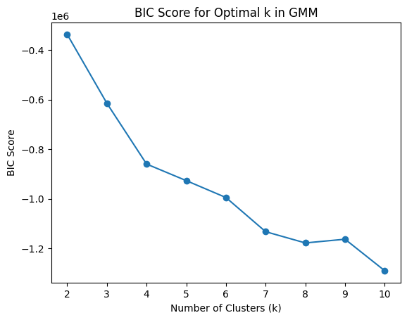
# prompt: can you find the best k for a GMM with elbow?

from sklearn.mixture import GaussianMixture

# Calculate BIC scores for different values of k
bic_scores = []
k_values = range(2, 11)  # Test k values from 2 to 20

scaler = StandardScaler()
scaled_data = scaler.fit_transform(data2)

for k in k_values:
    gmm = GaussianMixture(n_components=k, random_state=42, n_init=10)
    gmm.fit(scaled_data)  # Use scaled_data here
    bic_scores.append(gmm.bic(scaled_data))

# Find the best k based on the lowest BIC score
best_k = k_values[np.argmin(bic_scores)]
print(f"Best k based on BIC score: {best_k}")

# Plot the BIC scores
plt.plot(k_values, bic_scores, marker='o')
plt.xlabel('Number of Clusters (k)')
plt.ylabel('BIC Score')
plt.title('BIC Score for Optimal k in GMM')
plt.show()

Best k based on BIC score: 10

# prompt: effettua la silhouette analysis per k=range(1,6)
import matplotlib.cm as cm
import matplotlib.pyplot as plt
import numpy as np

from sklearn.cluster import KMeans
from sklearn.datasets import make_blobs
from sklearn.metrics import silhouette_samples, silhouette_score

# Calculate silhouette scores for different values of k
silhouette_scores = []
k_values = range(2, 6)  # Test k values from 2 to 5 (Silhouette score is not defined for k=1)

scaler = StandardScaler()
scaled_data = scaler.fit_transform(data2)

for k in k_values:
    gmm = GaussianMixture(n_components=k, random_state=42, n_init=10)
    gmm.fit(scaled_data)
    cluster_labels = pipeline.gmm(data2)
    silhouette_avg = silhouette_score(data2, cluster_labels) # Use data2 directly here
    silhouette_scores.append(silhouette_avg)
    sample_silhouette_values = silhouette_samples(data2, cluster_labels)

    fig, (ax1) = plt.subplots(1, 1)
    fig.set_size_inches(18, 7)


    # The 1st subplot is the silhouette plot
    # The silhouette coefficient can range from -1, 1 but in this example all
    # lie within [-0.1, 1]
    #ax1.set_xlim([-0.1, 1])
    # The (n_clusters+1)*10 is for inserting blank space between silhouette
    # plots of individual clusters, to demarcate them clearly.
    #ax1.set_ylim([0, len(data2) + (k + 1) * 10])

    y_lower = 10
    for i in range(k):
        # Aggregate the silhouette scores for samples belonging to
        # cluster i, and sort them
        ith_cluster_silhouette_values = sample_silhouette_values[cluster_labels == i]

        ith_cluster_silhouette_values.sort()

        size_cluster_i = ith_cluster_silhouette_values.shape[0]
        y_upper = y_lower + size_cluster_i

        color = cm.nipy_spectral(float(i) / k)
        ax1.fill_betweenx(
            np.arange(y_lower, y_upper),
            0,
            ith_cluster_silhouette_values,
            facecolor=color,
            edgecolor=color,
            alpha=0.7,
        )

        # Label the silhouette plots with their cluster numbers at the middle
        ax1.text(-0.05, y_lower + 0.5 * size_cluster_i, str(i))

        # Compute the new y_lower for next plot
        y_lower = y_upper + 10  # 10 for the 0 samples

    ax1.set_title(f"The silhouette plot for k={k}")
    ax1.set_xlabel("The silhouette coefficient values")
    ax1.set_ylabel("Cluster label")

    # The vertical line for average silhouette score of all the values
    ax1.axvline(x=silhouette_avg, color="red", linestyle="--")

    ax1.set_yticks([])  # Clear the yaxis labels / ticks
    ax1.set_xticks([-0.1, 0, 0.2, 0.4, 0.6, 0.8, 1])

# Find the best k based on the highest silhouette score
best_k = k_values[np.argmax(silhouette_scores)]
print(f"Best k based on Silhouette score: {best_k}")

# Plot the silhouette scores
plt.figure(figsize=(10, 6))
plt.plot(k_values, silhouette_scores, marker='o')
plt.xlabel('Number of Clusters (k)')
plt.ylabel('Silhouette Score')
plt.title('Silhouette Score for Optimal k')
plt.show()

Best k based on Silhouette score: 2

# prompt: fai pca sul dataset "data2" e mostra uno scree plot

import pandas as pd
import numpy as np
import matplotlib.pyplot as plt
from sklearn.decomposition import PCA
from sklearn.preprocessing import StandardScaler

# Assuming 'data2' is already defined as in your provided code
# ... (your existing code to define data2) ...

# Scale the data
scaler = StandardScaler()
scaled_data = scaler.fit_transform(data2)

# Apply PCA
pca = PCA()
pca.fit(scaled_data)

# Scree plot
plt.figure(figsize=(10, 6))
plt.plot(np.cumsum(pca.explained_variance_ratio_))
plt.xlabel('Number of Components')
plt.ylabel('Cumulative Explained Variance')
plt.title('Scree Plot')
plt.grid(True)
plt.show()

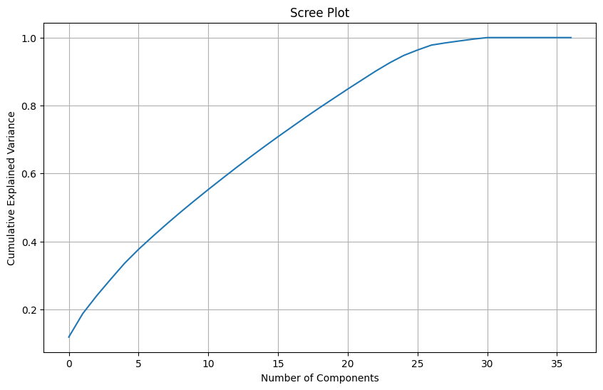
np.cumsum(pca.explained_variance_ratio_)[24]

0.9472334124009314

pca = PCA(n_components=25)
pca.fit(scaled_data)

x_pca = pca.transform(scaled_data)

# prompt: effettua la silhouette analysis per k=range(1,6)
import matplotlib.cm as cm
import matplotlib.pyplot as plt
import numpy as np

from sklearn.cluster import KMeans
from sklearn.datasets import make_blobs
from sklearn.metrics import silhouette_samples, silhouette_score

# Calculate silhouette scores for different values of k
silhouette_scores = []
k_values = range(2, 6)  # Test k values from 2 to 5 (Silhouette score is not defined for k=1)

pca = PCA()
pca.fit(scaled_data)

x_pca = pca.transform(scaled_data)

for k in k_values:
    kmeans = KMeans(n_clusters=k, n_init='auto', random_state=42)
    kmeans.fit(x_pca)

    cluster_labels = kmeans.predict(x_pca)
    silhouette_avg = silhouette_score(x_pca, cluster_labels) # Use data2 directly here
    silhouette_scores.append(silhouette_avg)
    sample_silhouette_values = silhouette_samples(x_pca, cluster_labels)

    fig, (ax1) = plt.subplots(1, 1)
    fig.set_size_inches(18, 7)


    # The 1st subplot is the silhouette plot
    # The silhouette coefficient can range from -1, 1 but in this example all
    # lie within [-0.1, 1]
    #ax1.set_xlim([-0.1, 1])
    # The (n_clusters+1)*10 is for inserting blank space between silhouette
    # plots of individual clusters, to demarcate them clearly.
    #ax1.set_ylim([0, len(data2) + (k + 1) * 10])

    y_lower = 10
    for i in range(k):
        # Aggregate the silhouette scores for samples belonging to
        # cluster i, and sort them
        ith_cluster_silhouette_values = sample_silhouette_values[cluster_labels == i]

        ith_cluster_silhouette_values.sort()

        size_cluster_i = ith_cluster_silhouette_values.shape[0]
        y_upper = y_lower + size_cluster_i

        color = cm.nipy_spectral(float(i) / k)
        ax1.fill_betweenx(
            np.arange(y_lower, y_upper),
            0,
            ith_cluster_silhouette_values,
            facecolor=color,
            edgecolor=color,
            alpha=0.7,
        )

        # Label the silhouette plots with their cluster numbers at the middle
        ax1.text(-0.05, y_lower + 0.5 * size_cluster_i, str(i))

        # Compute the new y_lower for next plot
        y_lower = y_upper + 10  # 10 for the 0 samples

    ax1.set_title(f"The silhouette plot for k={k}")
    ax1.set_xlabel("The silhouette coefficient values")
    ax1.set_ylabel("Cluster label")

    # The vertical line for average silhouette score of all the values
    ax1.axvline(x=silhouette_avg, color="red", linestyle="--")

    ax1.set_yticks([])  # Clear the yaxis labels / ticks
    ax1.set_xticks([-0.1, 0, 0.2, 0.4, 0.6, 0.8, 1])

# Find the best k based on the highest silhouette score
best_k = k_values[np.argmax(silhouette_scores)]
print(f"Best k based on Silhouette score: {best_k}")

# Plot the silhouette scores
plt.figure(figsize=(10, 6))
plt.plot(k_values, silhouette_scores, marker='o')
plt.xlabel('Number of Clusters (k)')
plt.ylabel('Silhouette Score')
plt.title('Silhouette Score for Optimal k')
plt.show()

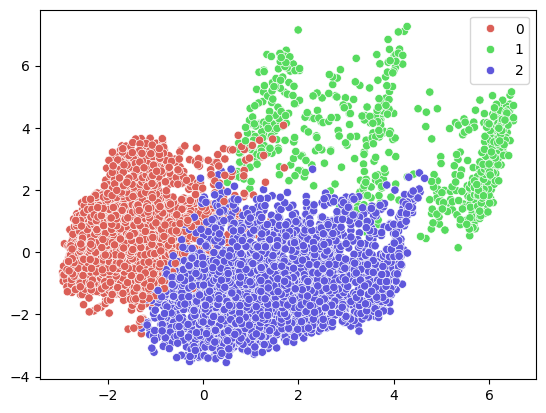
Best k based on Silhouette score: 3

import seaborn as sns

kmeans = KMeans(n_clusters=3, n_init='auto', random_state=42)
kmeans.fit(x_pca)

cluster_labels = kmeans.predict(x_pca)

sns.scatterplot(x=x_pca[:,0], y=x_pca[:,1], hue = cluster_labels, palette=sns.color_palette('hls', 3))

<Axes: >

data2['cluster'] = cluster_labels

data['cluster'] = cluster_labels

(np.cov(x_pca.T)*100).astype(np.int32)

array([[438,   0,   0, ...,   0,   0,   0],
       [  0, 255,   0, ...,   0,   0,   0],
       [  0,   0, 194, ...,   0,   0,   0],
       ...,
       [  0,   0,   0, ...,   0,   0,   0],
       [  0,   0,   0, ...,   0,   0,   0],
       [  0,   0,   0, ...,   0,   0,   0]], dtype=int32)

x_pca[:,[0,1]].shape

(10127, 2)

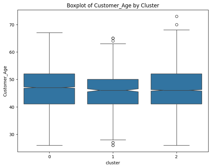
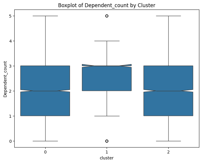
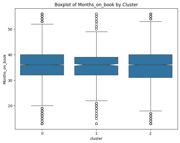
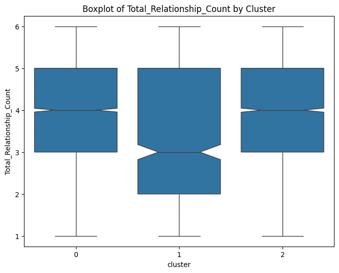
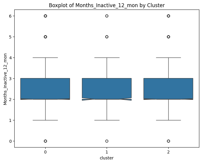
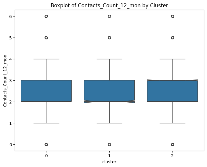
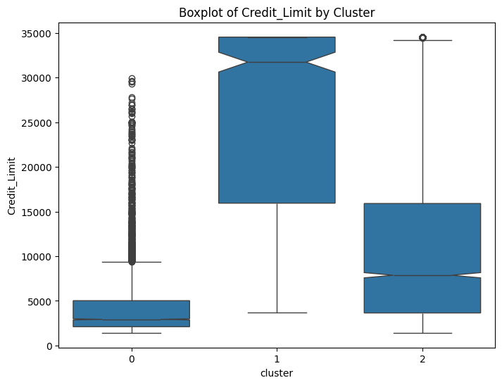
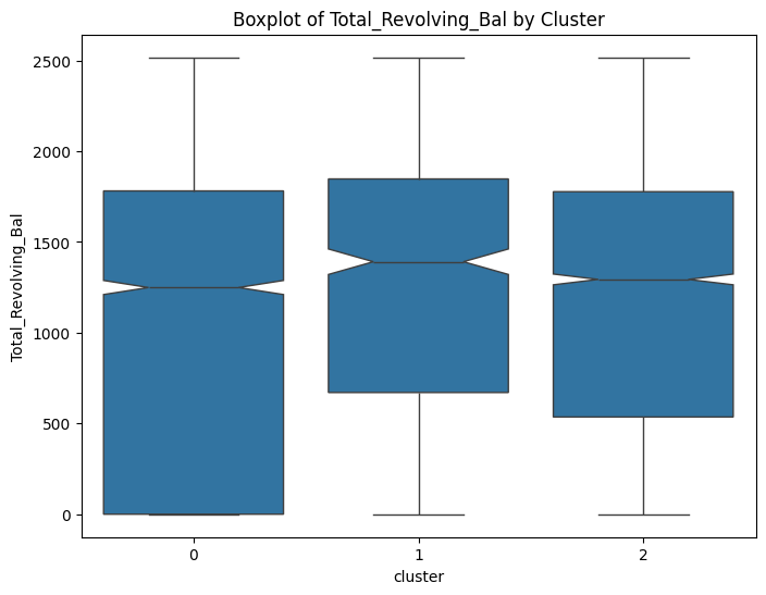
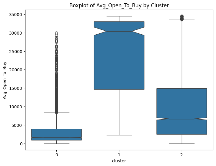
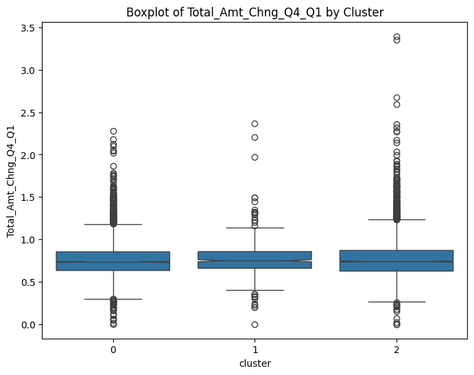
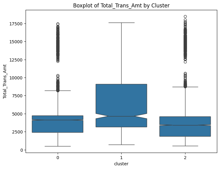
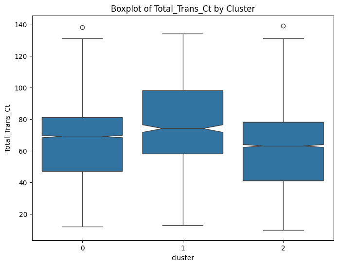
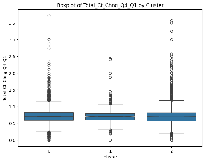
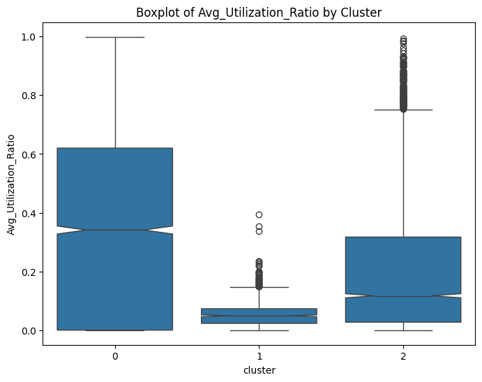
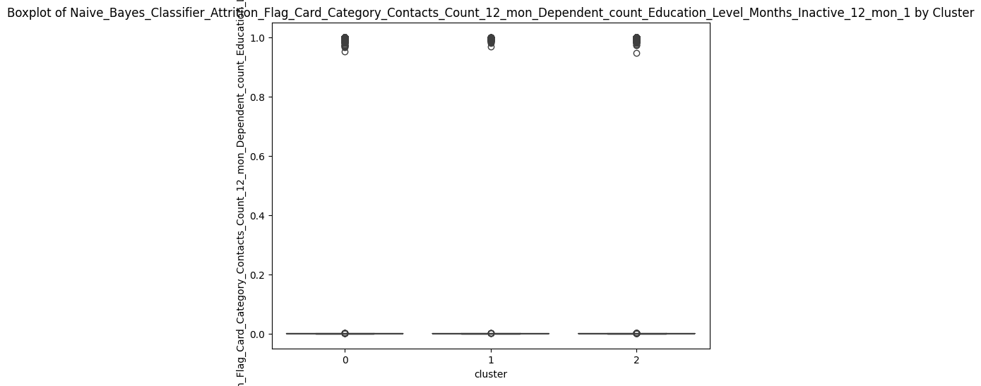
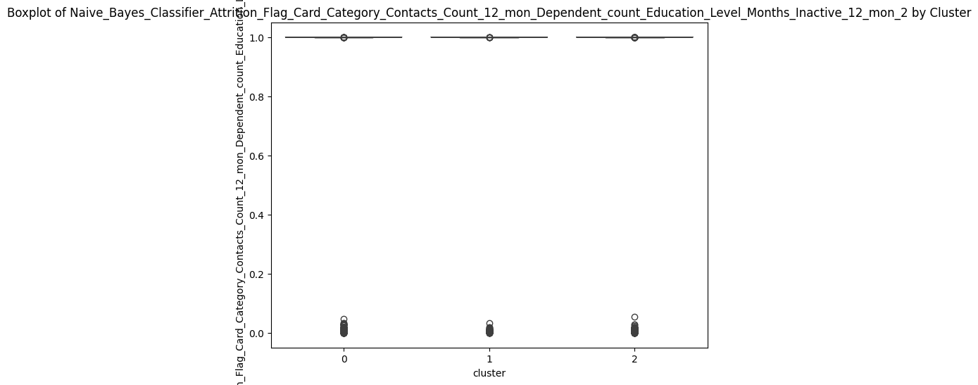
# prompt: can you plot boxplots for numeric variables in data2 grouped by cluster?

import matplotlib.pyplot as plt
import seaborn as sns

# Assuming 'data2' and 'cluster_labels' are already defined from your previous code
# ... (your existing code to define data2 and cluster_labels) ...

# Select numeric columns for boxplots
numeric_cols = data.select_dtypes(include=['number']).columns

# Create boxplots for each numeric variable grouped by cluster
for col in numeric_cols:
  plt.figure(figsize=(8, 6))
  sns.boxplot(x='cluster', y=col, data=data, notch=True)
  plt.title(f'Boxplot of {col} by Cluster')
  plt.show()

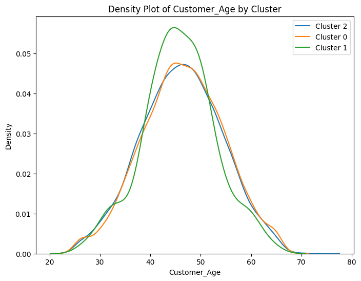
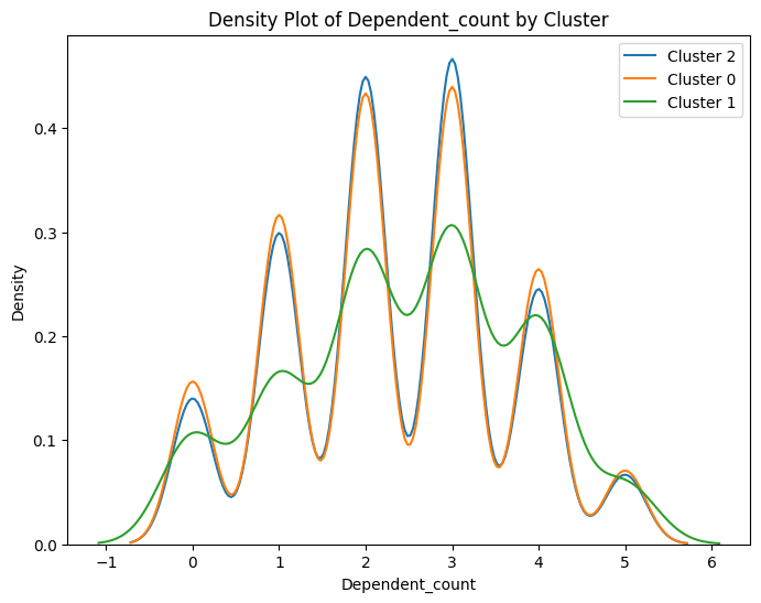
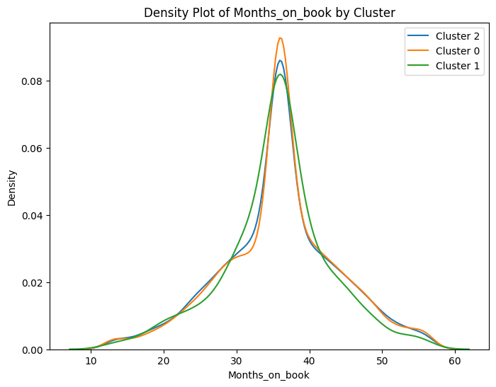
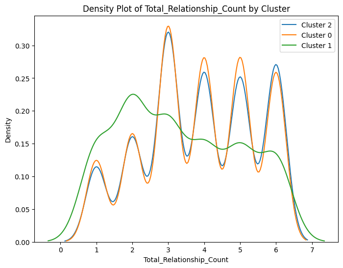
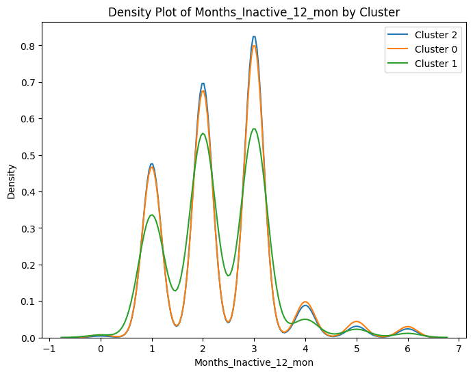
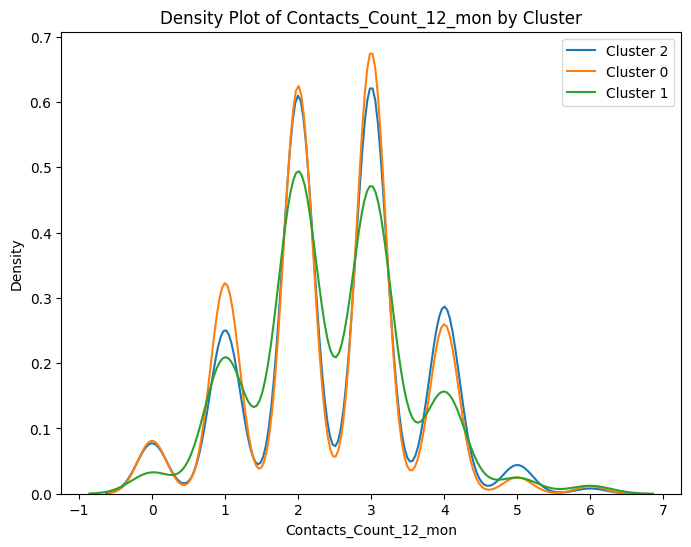
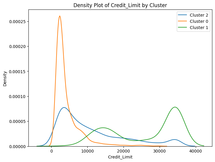
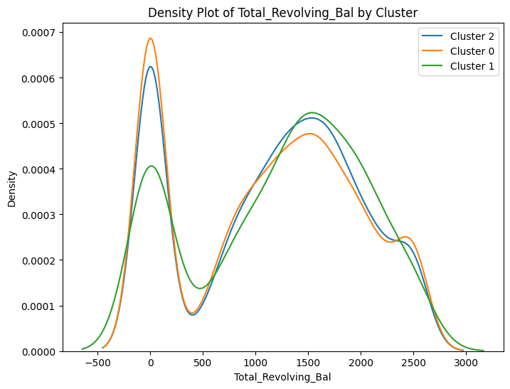
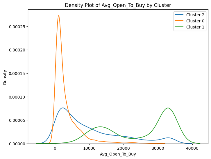
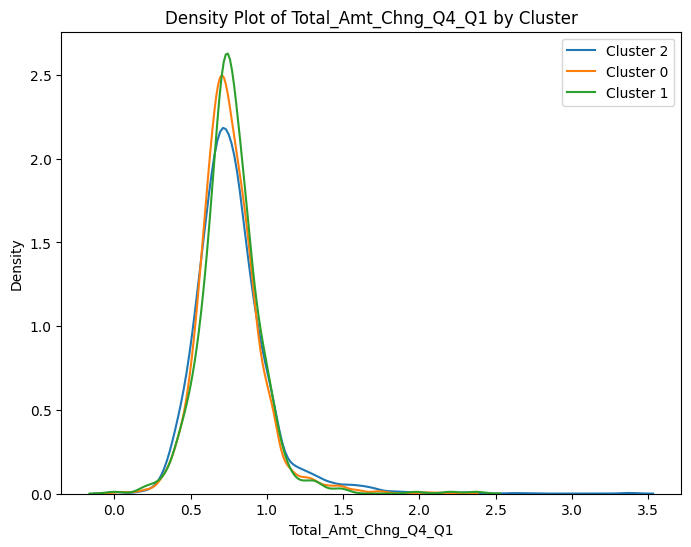
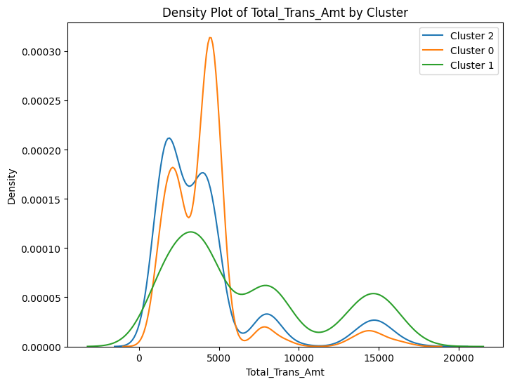
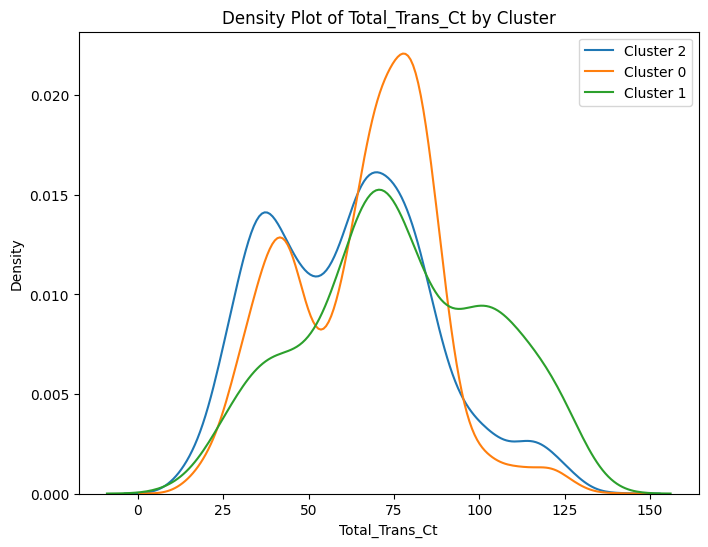
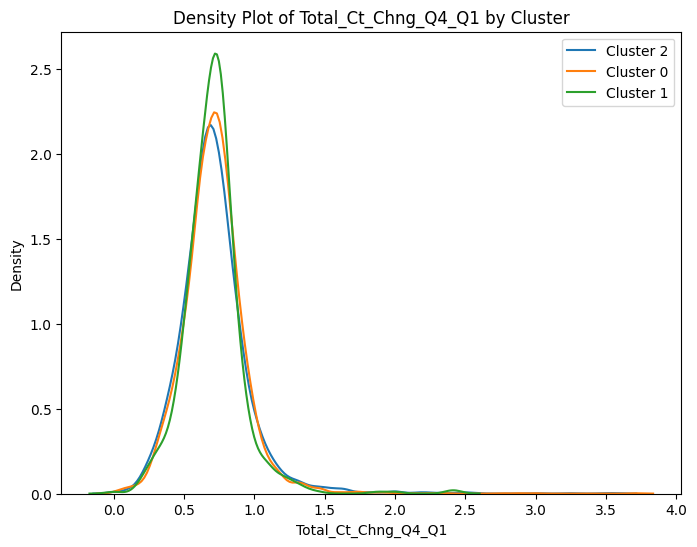
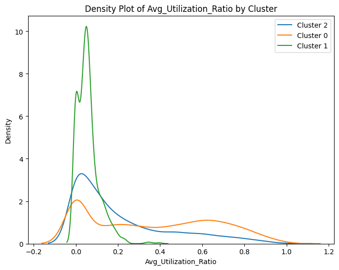
# prompt: can you plot density estimates for numeric variables in data2 grouped by cluster?

# Assuming 'data2' and 'cluster_labels' are already defined from your previous code
# ... (your existing code to define data2 and cluster_labels) ...

# Select numeric columns for density plots
numeric_cols = data2.select_dtypes(include=['number']).columns

# Create density plots for each numeric variable grouped by cluster
for col in numeric_cols:
    plt.figure(figsize=(8, 6))
    for cluster in data2['cluster'].unique():
        sns.kdeplot(data2[data2['cluster'] == cluster][col], label=f'Cluster {cluster}')
    plt.title(f'Density Plot of {col} by Cluster')
    plt.xlabel(col)
    plt.ylabel('Density')
    plt.legend()
    plt.show()

<ipython-input-100-ccc587c35145>:13: UserWarning: Dataset has 0 variance; skipping density estimate. Pass `warn_singular=False` to disable this warning.
  sns.kdeplot(data2[data2['cluster'] == cluster][col], label=f'Cluster {cluster}')
<ipython-input-100-ccc587c35145>:13: UserWarning: Dataset has 0 variance; skipping density estimate. Pass `warn_singular=False` to disable this warning.
  sns.kdeplot(data2[data2['cluster'] == cluster][col], label=f'Cluster {cluster}')
<ipython-input-100-ccc587c35145>:13: UserWarning: Dataset has 0 variance; skipping density estimate. Pass `warn_singular=False` to disable this warning.
  sns.kdeplot(data2[data2['cluster'] == cluster][col], label=f'Cluster {cluster}')
WARNING:matplotlib.legend:No artists with labels found to put in legend.  Note that artists whose label start with an underscore are ignored when legend() is called with no argument.