29. Exploratory Analysis on the Heart Disease Dataset

# This Python 3 environment comes with many helpful analytics libraries installed
# It is defined by the kaggle/python Docker image: https://github.com/kaggle/docker-python
# For example, here's several helpful packages to load

import numpy as np # linear algebra
import pandas as pd # data processing, CSV file I/O (e.g. pd.read_csv)

# Input data files are available in the read-only "../input/" directory
# For example, running this (by clicking run or pressing Shift+Enter) will list all files under the input directory

import os
for dirname, _, filenames in os.walk('/kaggle/input'):
    for filename in filenames:
        print(os.path.join(dirname, filename))

# You can write up to 20GB to the current directory (/kaggle/working/) that gets preserved as output when you create a version using "Save & Run All" 
# You can also write temporary files to /kaggle/temp/, but they won't be saved outside of the current session

import pandas as pd
#Alternatively: download data from https://www.kaggle.com/datasets/redwankarimsony/heart-disease-data
df = pd.read_csv('/kaggle/input/heart-disease-data/heart_disease_uci.csv')
df.head(10)

	id	age	sex	dataset	cp	trestbps	chol	fbs	restecg	thalch	exang	oldpeak	slope	ca	thal	num
0	1	63	Male	Cleveland	typical angina	145.0	233.0	True	lv hypertrophy	150.0	False	2.3	downsloping	0.0	fixed defect	0
1	2	67	Male	Cleveland	asymptomatic	160.0	286.0	False	lv hypertrophy	108.0	True	1.5	flat	3.0	normal	2
2	3	67	Male	Cleveland	asymptomatic	120.0	229.0	False	lv hypertrophy	129.0	True	2.6	flat	2.0	reversable defect	1
3	4	37	Male	Cleveland	non-anginal	130.0	250.0	False	normal	187.0	False	3.5	downsloping	0.0	normal	0
4	5	41	Female	Cleveland	atypical angina	130.0	204.0	False	lv hypertrophy	172.0	False	1.4	upsloping	0.0	normal	0
5	6	56	Male	Cleveland	atypical angina	120.0	236.0	False	normal	178.0	False	0.8	upsloping	0.0	normal	0
6	7	62	Female	Cleveland	asymptomatic	140.0	268.0	False	lv hypertrophy	160.0	False	3.6	downsloping	2.0	normal	3
7	8	57	Female	Cleveland	asymptomatic	120.0	354.0	False	normal	163.0	True	0.6	upsloping	0.0	normal	0
8	9	63	Male	Cleveland	asymptomatic	130.0	254.0	False	lv hypertrophy	147.0	False	1.4	flat	1.0	reversable defect	2
9	10	53	Male	Cleveland	asymptomatic	140.0	203.0	True	lv hypertrophy	155.0	True	3.1	downsloping	0.0	reversable defect	1

df = df.set_index('id')
df

	age	sex	dataset	cp	trestbps	chol	fbs	restecg	thalch	exang	oldpeak	slope	ca	thal	num
id
1	63	Male	Cleveland	typical angina	145.0	233.0	True	lv hypertrophy	150.0	False	2.3	downsloping	0.0	fixed defect	0
2	67	Male	Cleveland	asymptomatic	160.0	286.0	False	lv hypertrophy	108.0	True	1.5	flat	3.0	normal	2
3	67	Male	Cleveland	asymptomatic	120.0	229.0	False	lv hypertrophy	129.0	True	2.6	flat	2.0	reversable defect	1
4	37	Male	Cleveland	non-anginal	130.0	250.0	False	normal	187.0	False	3.5	downsloping	0.0	normal	0
5	41	Female	Cleveland	atypical angina	130.0	204.0	False	lv hypertrophy	172.0	False	1.4	upsloping	0.0	normal	0
...	...	...	...	...	...	...	...	...	...	...	...	...	...	...	...
916	54	Female	VA Long Beach	asymptomatic	127.0	333.0	True	st-t abnormality	154.0	False	0.0	NaN	NaN	NaN	1
917	62	Male	VA Long Beach	typical angina	NaN	139.0	False	st-t abnormality	NaN	NaN	NaN	NaN	NaN	NaN	0
918	55	Male	VA Long Beach	asymptomatic	122.0	223.0	True	st-t abnormality	100.0	False	0.0	NaN	NaN	fixed defect	2
919	58	Male	VA Long Beach	asymptomatic	NaN	385.0	True	lv hypertrophy	NaN	NaN	NaN	NaN	NaN	NaN	0
920	62	Male	VA Long Beach	atypical angina	120.0	254.0	False	lv hypertrophy	93.0	True	0.0	NaN	NaN	NaN	1

920 rows × 15 columns

df.info()

<class 'pandas.core.frame.DataFrame'>
RangeIndex: 303 entries, 0 to 302
Data columns (total 14 columns):
 #   Column    Non-Null Count  Dtype  
---  ------    --------------  -----  
 0   age       303 non-null    int64  
 1   sex       303 non-null    int64  
 2   cp        303 non-null    int64  
 3   trestbps  303 non-null    int64  
 4   chol      303 non-null    int64  
 5   fbs       303 non-null    int64  
 6   restecg   303 non-null    int64  
 7   thalach   303 non-null    int64  
 8   exang     303 non-null    int64  
 9   oldpeak   303 non-null    float64
 10  slope     303 non-null    int64  
 11  ca        299 non-null    float64
 12  thal      301 non-null    float64
 13  num       303 non-null    int64  
dtypes: float64(3), int64(11)
memory usage: 33.3 KB

29.1. Descriptive Analysis

Let’s see the statistic summary:

df.describe()

	id	age	trestbps	chol	thalch	oldpeak	ca	num
count	920.000000	920.000000	861.000000	890.000000	865.000000	858.000000	309.000000	920.000000
mean	460.500000	53.510870	132.132404	199.130337	137.545665	0.878788	0.676375	0.995652
std	265.725422	9.424685	19.066070	110.780810	25.926276	1.091226	0.935653	1.142693
min	1.000000	28.000000	0.000000	0.000000	60.000000	-2.600000	0.000000	0.000000
25%	230.750000	47.000000	120.000000	175.000000	120.000000	0.000000	0.000000	0.000000
50%	460.500000	54.000000	130.000000	223.000000	140.000000	0.500000	0.000000	1.000000
75%	690.250000	60.000000	140.000000	268.000000	157.000000	1.500000	1.000000	2.000000
max	920.000000	77.000000	200.000000	603.000000	202.000000	6.200000	3.000000	4.000000

df['dataset'].unique()

array(['Cleveland', 'Hungary', 'Switzerland', 'VA Long Beach'],
      dtype=object)

df['slope'].unique()

array(['downsloping', 'flat', 'upsloping', nan], dtype=object)

Let’s visualize all plots in different scales:numeric_columns

from matplotlib import pyplot as plt
#select numeric columns
numeric_columns = df.select_dtypes(include='number').columns #remove first column id
n = len(numeric_columns)
plt.figure(figsize=(12,4))
for i,var in enumerate(numeric_columns):
    plt.subplot(1,n,i+1)
    df[var].plot.box()

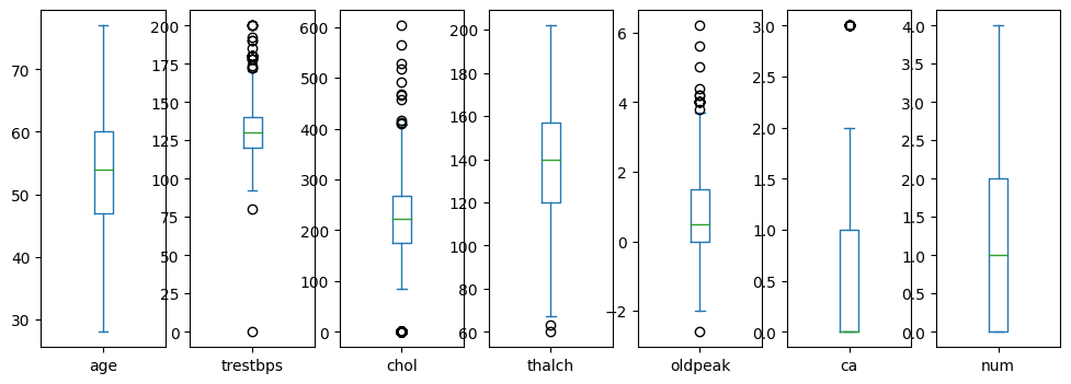
Age looks well distributed. trestbps, chol, thalch, oldpeak have outliers.

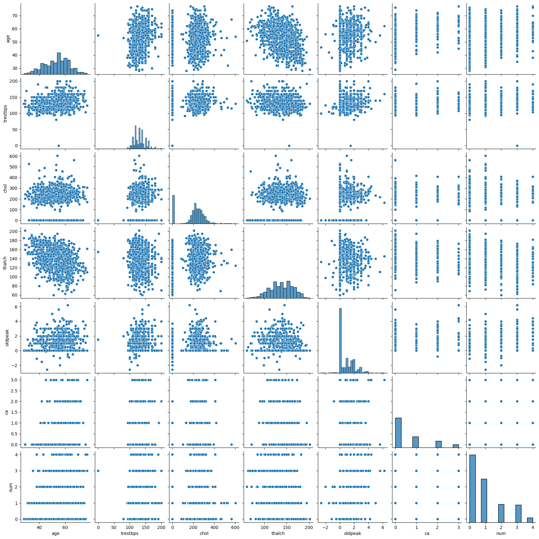
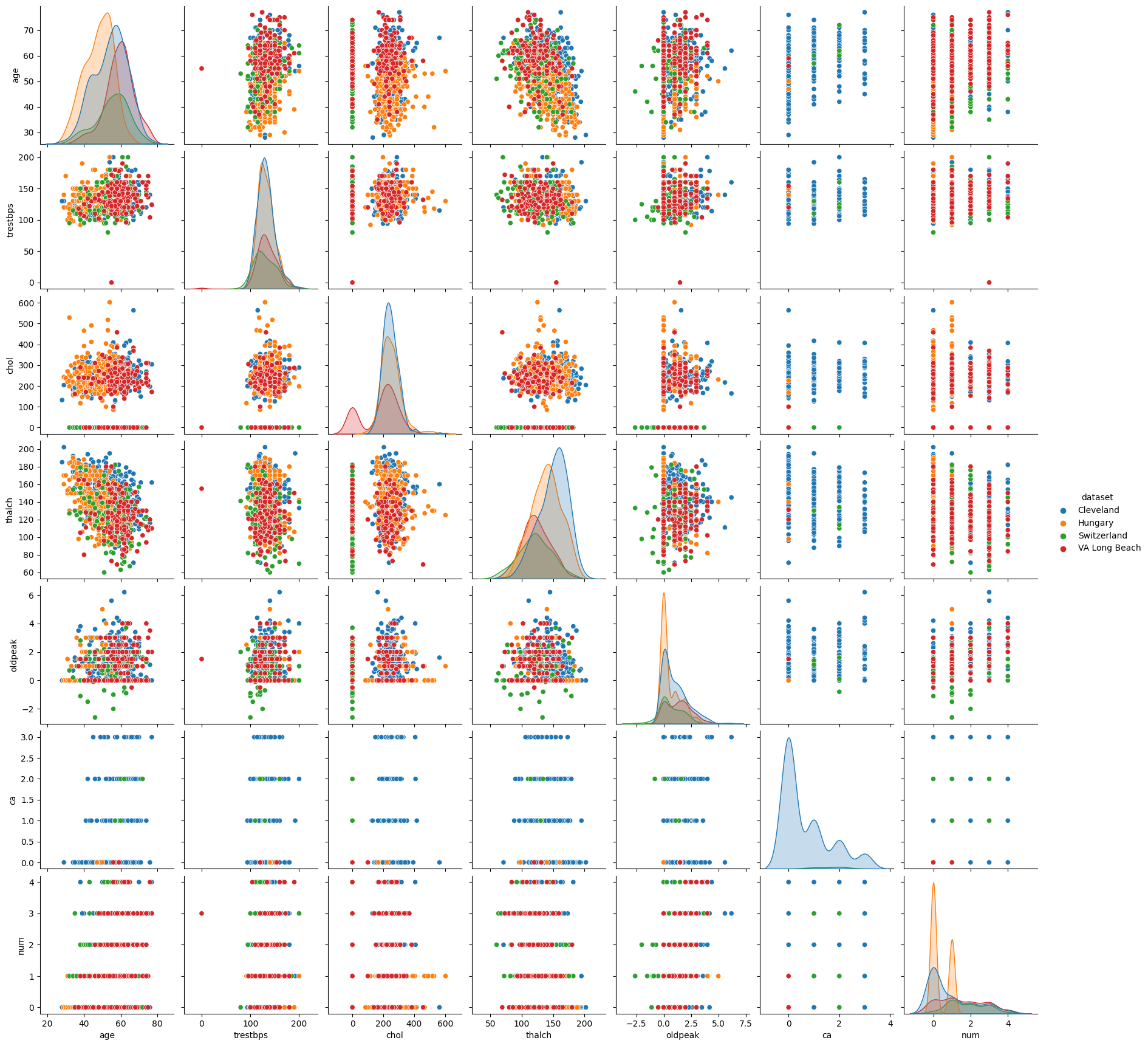
import seaborn as sns
sns.pairplot(df.select_dtypes(include='number'))

/opt/conda/lib/python3.10/site-packages/seaborn/axisgrid.py:118: UserWarning: The figure layout has changed to tight
  self._figure.tight_layout(*args, **kwargs)

<seaborn.axisgrid.PairGrid at 0x7f263033dc90>

df.select_dtypes(include='number').columns

Index(['age', 'trestbps', 'chol', 'thalch', 'oldpeak', 'ca', 'num'], dtype='object')

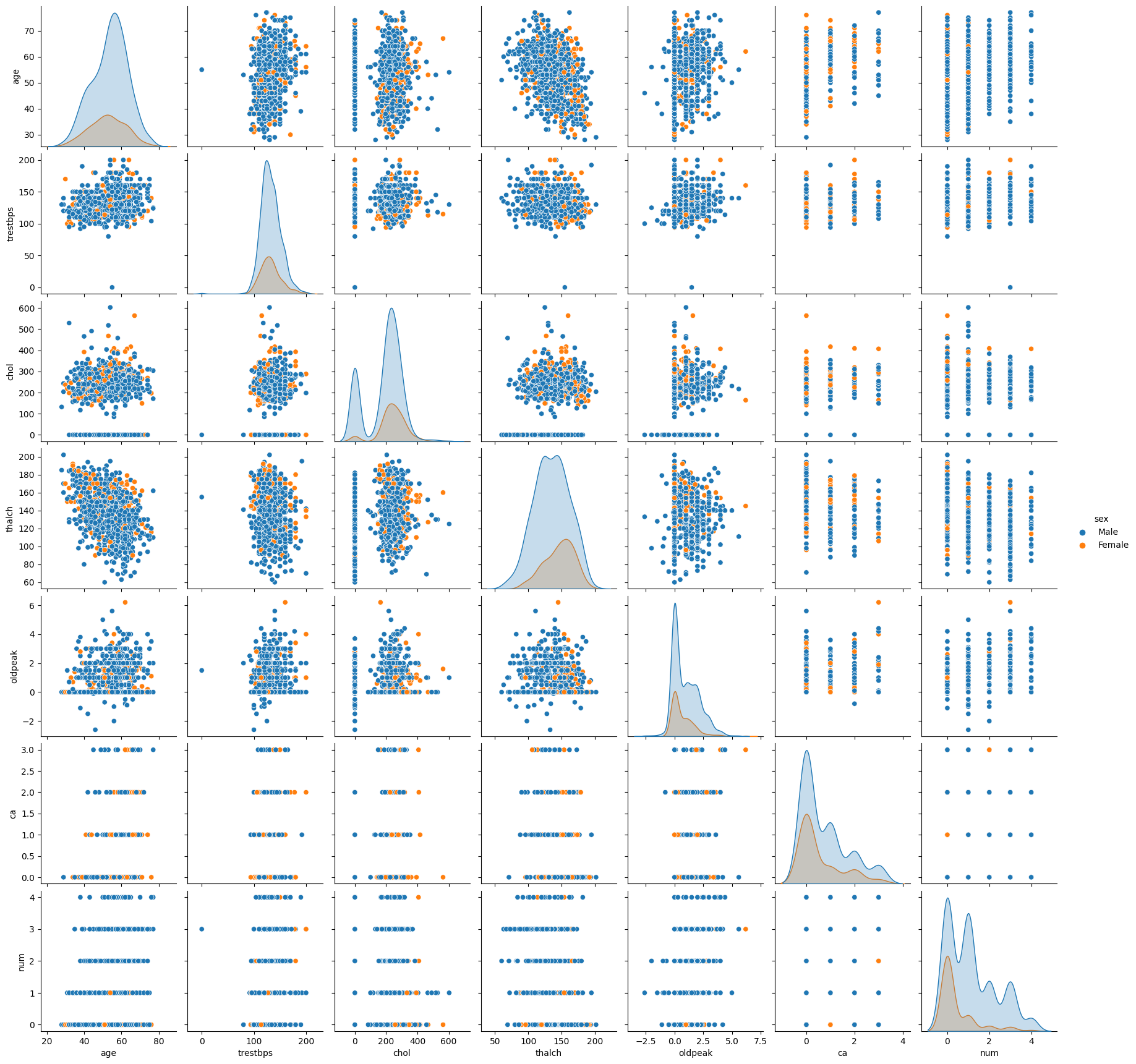
columns = ['age', 'trestbps', 'chol', 'thalch', 'oldpeak', 'ca', 'num','sex']
sns.pairplot(df[columns], hue='sex')

/opt/conda/lib/python3.10/site-packages/seaborn/axisgrid.py:118: UserWarning: The figure layout has changed to tight
  self._figure.tight_layout(*args, **kwargs)

<seaborn.axisgrid.PairGrid at 0x7f260a140640>

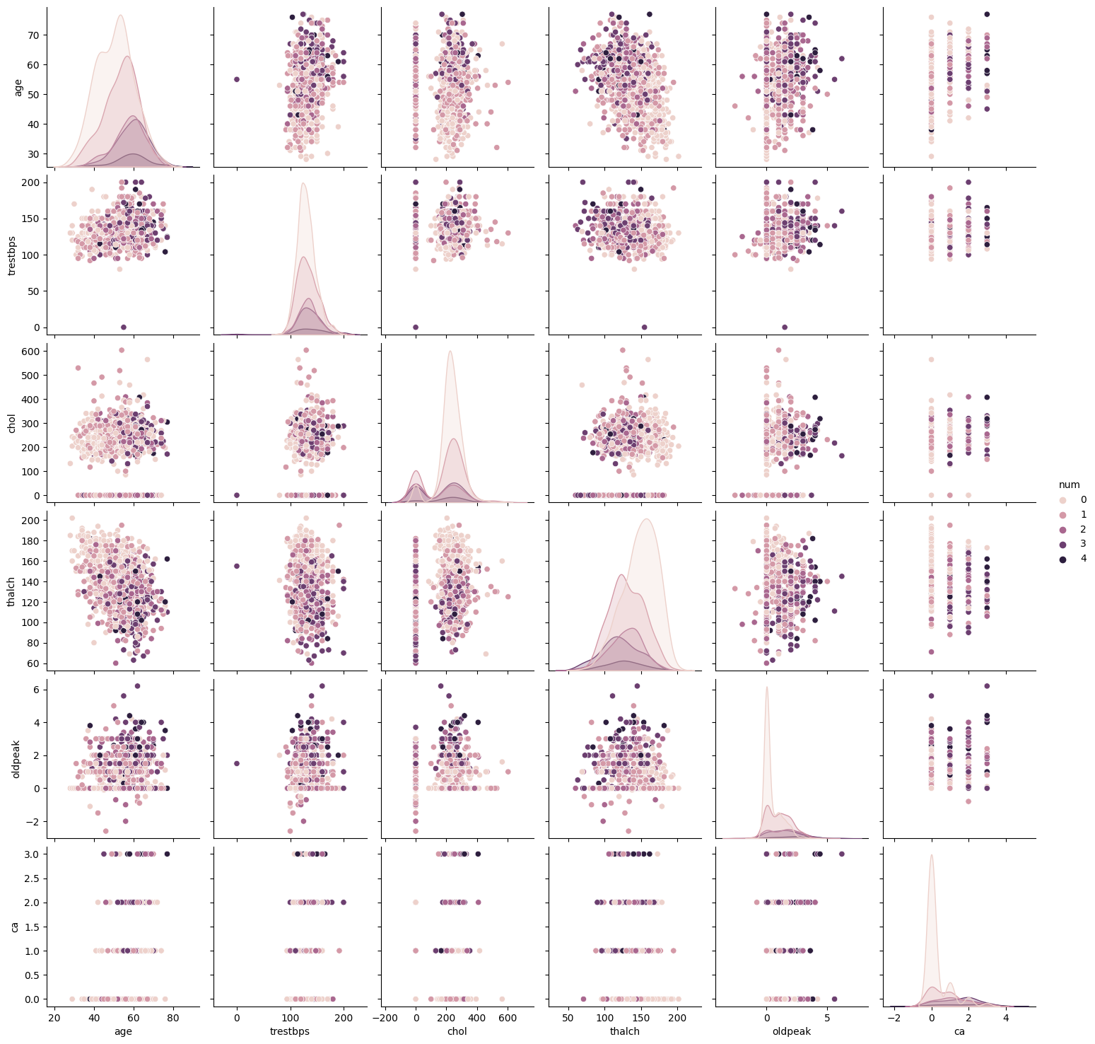
columns = ['age', 'trestbps', 'chol', 'thalch', 'oldpeak', 'ca', 'num']
sns.pairplot(df[columns], hue='num')

/opt/conda/lib/python3.10/site-packages/seaborn/axisgrid.py:118: UserWarning: The figure layout has changed to tight
  self._figure.tight_layout(*args, **kwargs)

<seaborn.axisgrid.PairGrid at 0x7f26081bdc60>

columns = ['age', 'trestbps', 'chol', 'thalch', 'oldpeak', 'ca', 'num','dataset']
sns.pairplot(df[columns], hue='dataset')

/opt/conda/lib/python3.10/site-packages/seaborn/axisgrid.py:118: UserWarning: The figure layout has changed to tight
  self._figure.tight_layout(*args, **kwargs)

<seaborn.axisgrid.PairGrid at 0x7f260696f490>

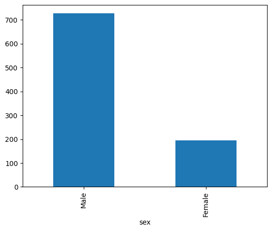
df['sex'].value_counts().plot.bar()

<Axes: xlabel='sex'>

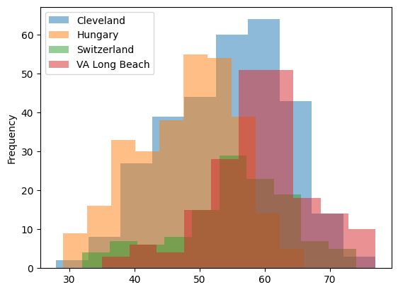
29.2. Is the dataset balanced across sites?

df.groupby('dataset')['age'].plot.hist(alpha=0.5)
plt.legend()

<matplotlib.legend.Legend at 0x7f262028e6e0>

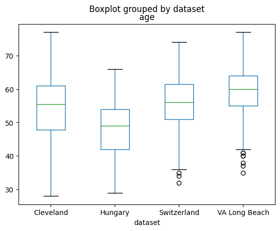
df.boxplot(column='age', by='dataset', grid=False)

<Axes: title={'center': 'age'}, xlabel='dataset'>

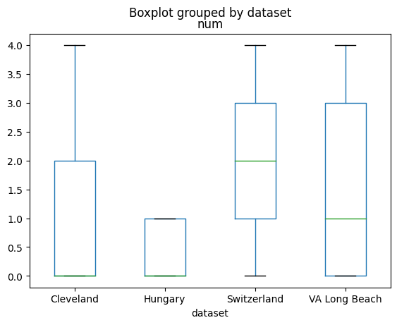
df.boxplot(column='num', by='dataset', grid=False)

<Axes: title={'center': 'num'}, xlabel='dataset'>

pd.crosstab(df['sex'],df['dataset'],normalize=1).T.plot.bar(stacked=True)

<Axes: xlabel='dataset'>

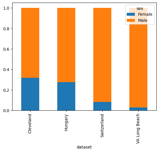
The data is not balanced with respect to sex and age across the three sites.

29.3. Is sex a risk factor for heart disease

pd.crosstab(df['num'],df['sex'], margins=True)

sex	Female	Male	All
num
0	144	267	411
1	30	235	265
2	10	99	109
3	8	99	107
4	2	26	28
All	194	726	920

pd.crosstab(df['num'],df['sex'], margins=True, normalize=1)

sex	Female	Male	All
num
0	0.742268	0.367769	0.446739
1	0.154639	0.323691	0.288043
2	0.051546	0.136364	0.118478
3	0.041237	0.136364	0.116304
4	0.010309	0.035813	0.030435

pd.crosstab(df['num'],df['sex'], margins=True, normalize=1).T.plot.bar(stacked=True)

<Axes: xlabel='sex'>

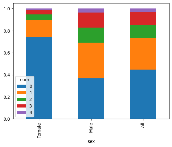
It looks like there is a correlation between the sex and num variables. Let’s measure the Pearson Chi2 statistic:

from scipy.stats import chi2_contingency
chi2_contingency(pd.crosstab(df['num'],df['sex'])).statistic

87.72950473296471

Let’s compare the expected frequencies with the observed ones:

pd.crosstab(df['num'],df['sex'])

sex	Female	Male
num
0	144	267
1	30	235
2	10	99
3	8	99
4	2	26

chi2_contingency(pd.crosstab(df['num'],df['sex'])).expected_freq

array([[ 86.6673913 , 324.3326087 ],
       [ 55.88043478, 209.11956522],
       [ 22.98478261,  86.01521739],
       [ 22.56304348,  84.43695652],
       [  5.90434783,  22.09565217]])

Let’s compute the Cramer V statistic, which is normalized:

from scipy.stats.contingency import association
association(pd.crosstab(df['num'],df['sex']))

0.30880116145902026

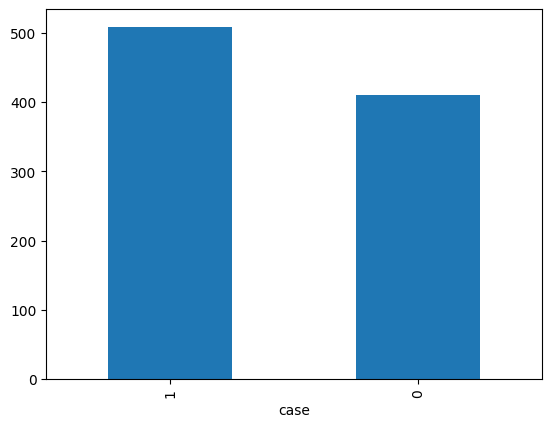
Let’s compute the relative risk to have a result which is easier to interpret:

df['case'] = (df['num']>0).astype(int)
df['case'].value_counts().plot.bar()

<Axes: xlabel='case'>

contingency = pd.crosstab(df['case'], df['sex'])
contingency.iloc[[1,0]][['Male','Female']]

sex	Male	Female
case
1	459	50
0	267	144

contingency['Female'][1]

50

from scipy.stats.contingency import relative_risk
relative_risk(contingency['Male'][1],contingency['Male'].sum(),contingency['Female'][1],contingency['Female'].sum()).relative_risk

2.4530578512396697

Let’s compute the odds ratio:

from scipy.stats.contingency import odds_ratio
odds_ratio(contingency.iloc[[1,0]][['Male','Female']])

OddsRatioResult(statistic=4.942016985387771)

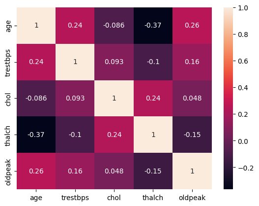
29.4. Are there correlations among the numerical variables?

pd.crosstab(df['num'],df['ca'])

ca	0.0	1.0	2.0	3.0
num
0	133	21	8	3
1	28	20	7	3
2	9	14	9	4
3	8	9	15	5
4	3	3	2	5

sns.heatmap(df.select_dtypes(include='number').drop(['case','num','ca'],axis=1).corr(), annot=True)

<Axes: >

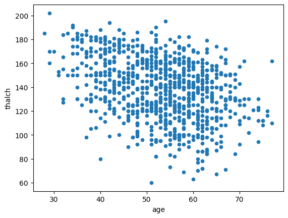
df.plot.scatter(x='age',y='thalch')

<Axes: xlabel='age', ylabel='thalch'>

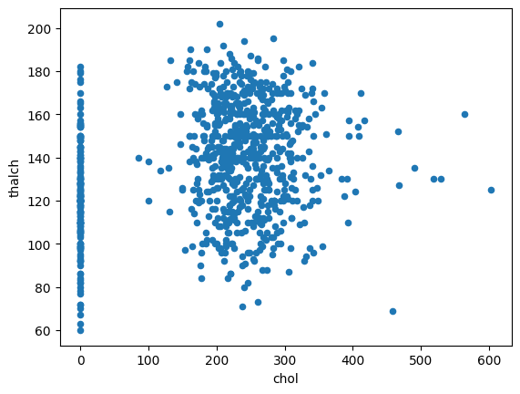
df.plot.scatter(x='chol',y='thalch')

<Axes: xlabel='chol', ylabel='thalch'>

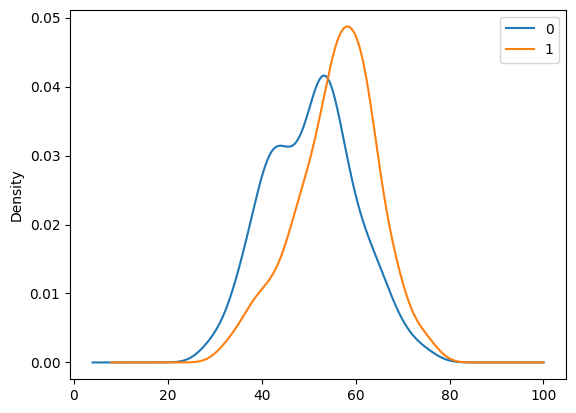
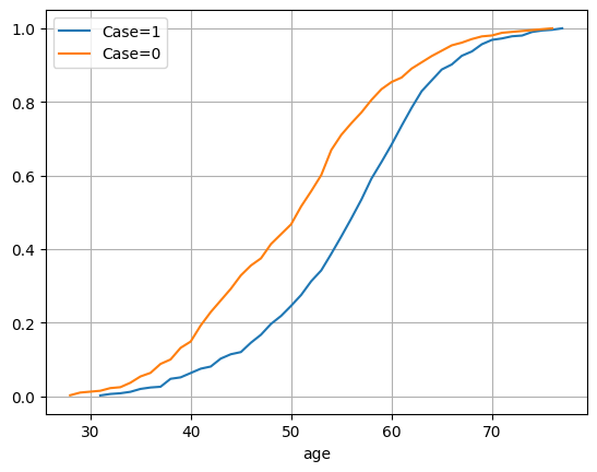
29.5. Is age is a risk factor?

df.groupby('case')['age'].plot.density()
plt.legend()

<matplotlib.legend.Legend at 0x7f26080cf5b0>

df_case = df[df['case']==1]
df_nocase = df[df['case']==0]

df_case['age'].value_counts(normalize=True).sort_index().cumsum().plot(label='Case=1')
df_nocase['age'].value_counts(normalize=True).sort_index().cumsum().plot(label='Case=0')
plt.legend()
plt.grid()

pd.cut(df['age'], bins=5)

id
1        (57.4, 67.2]
2        (57.4, 67.2]
3        (57.4, 67.2]
4      (27.951, 37.8]
5        (37.8, 47.6]
            ...      
916      (47.6, 57.4]
917      (57.4, 67.2]
918      (47.6, 57.4]
919      (57.4, 67.2]
920      (57.4, 67.2]
Name: age, Length: 920, dtype: category
Categories (5, interval[float64, right]): [(27.951, 37.8] < (37.8, 47.6] < (47.6, 57.4] < (57.4, 67.2] < (67.2, 77.0]]

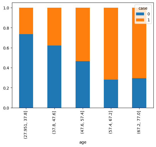
pd.crosstab(df['case'], pd.cut(df['age'], bins=5), normalize=1).T.plot.bar(stacked=True)

<Axes: xlabel='age'>

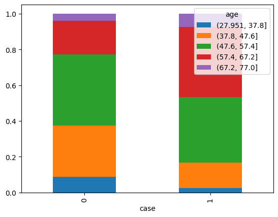
pd.crosstab(df['case'], pd.cut(df['age'], bins=5), normalize=0).plot.bar(stacked=True)

<Axes: xlabel='case'>

pd.crosstab(df['case'], pd.cut(df['age'], bins=2), normalize=0).plot.bar(stacked=True)

<Axes: xlabel='case'>

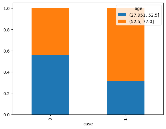
contingency = pd.crosstab(df['case'], pd.cut(df['age'], bins=2))
odds_ratio(contingency)

OddsRatioResult(statistic=2.766499032279526)

contingency

age	(27.951, 52.5]	(52.5, 77.0]
case
0	229	182
1	159	350