33. Linear and Logistic Regression Laboratory#
33.1. Linear Regression#
We will use the datatset available at this URL:
https://www.kaggle.com/datasets/yasserh/advertising-sales-dataset
Let us load the dataset:
import pandas as pd
advertising=pd.read_csv('Advertising Budget and Sales.csv')
advertising=advertising.rename(columns={
    'Unnamed: 0':'Index',
    'TV Ad Budget ($)': 'tv',
    'Radio Ad Budget ($)': 'radio',
    'Newspaper Ad Budget ($)': 'newspaper',
    'Sales ($)': 'sales'
    })
advertising.set_index('Index')
| tv | radio | newspaper | sales | |
|---|---|---|---|---|
| Index | ||||
| 1 | 230.1 | 37.8 | 69.2 | 22.1 |
| 2 | 44.5 | 39.3 | 45.1 | 10.4 |
| 3 | 17.2 | 45.9 | 69.3 | 9.3 |
| 4 | 151.5 | 41.3 | 58.5 | 18.5 |
| 5 | 180.8 | 10.8 | 58.4 | 12.9 |
| ... | ... | ... | ... | ... |
| 196 | 38.2 | 3.7 | 13.8 | 7.6 |
| 197 | 94.2 | 4.9 | 8.1 | 9.7 |
| 198 | 177.0 | 9.3 | 6.4 | 12.8 |
| 199 | 283.6 | 42.0 | 66.2 | 25.5 |
| 200 | 232.1 | 8.6 | 8.7 | 13.4 |
200 rows × 4 columns
advertising.info()
<class 'pandas.core.frame.DataFrame'>
RangeIndex: 200 entries, 0 to 199
Data columns (total 5 columns):
 #   Column     Non-Null Count  Dtype
---  ------     --------------  -----
 0   Index      200 non-null    int64
 1   tv         200 non-null    float64
 2   radio      200 non-null    float64
 3   newspaper  200 non-null    float64
 4   sales      200 non-null    float64
dtypes: float64(4), int64(1)
memory usage: 7.9 KB
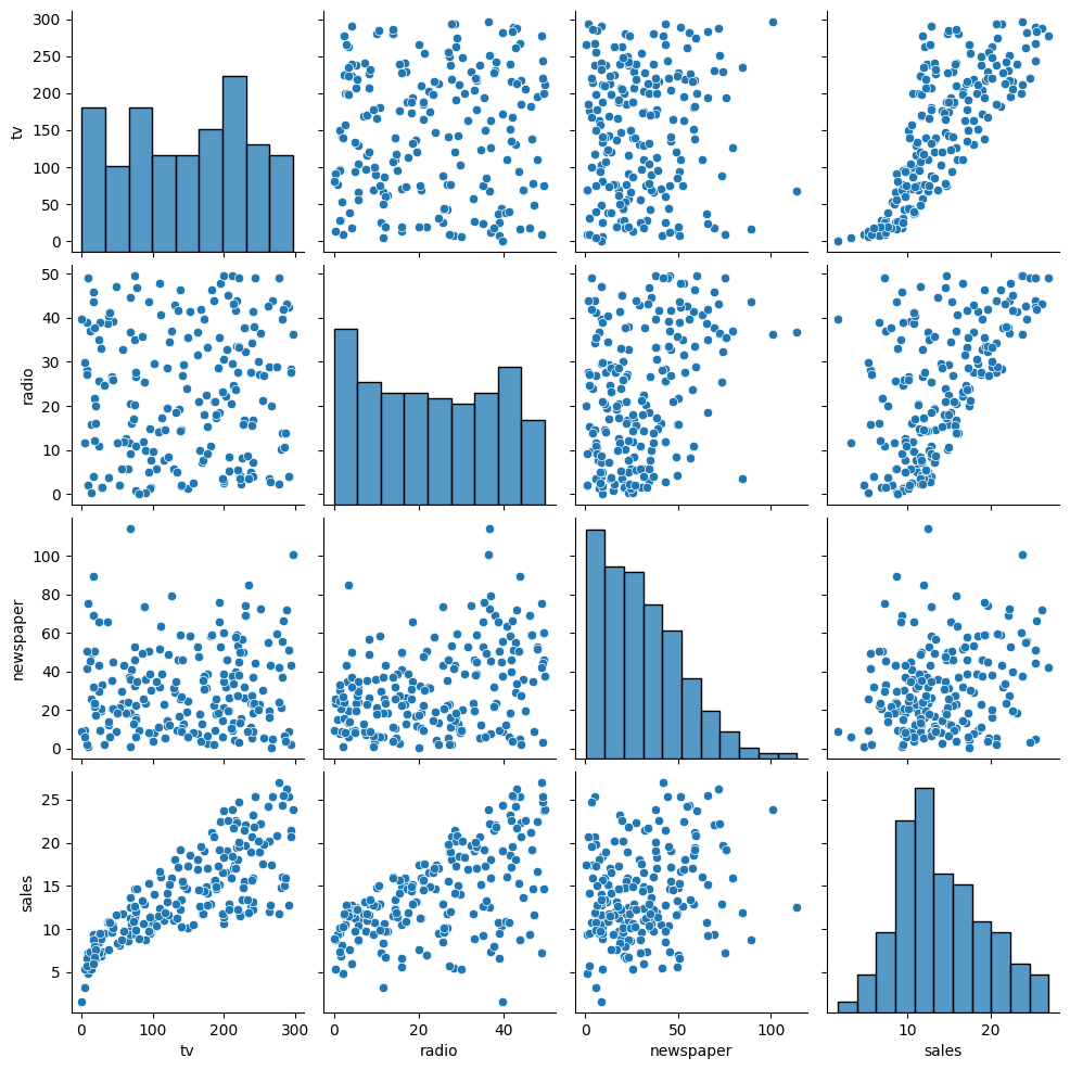
import seaborn as sns
sns.pairplot(advertising.drop('Index',axis=1))
<seaborn.axisgrid.PairGrid at 0x7b57ba39b460>
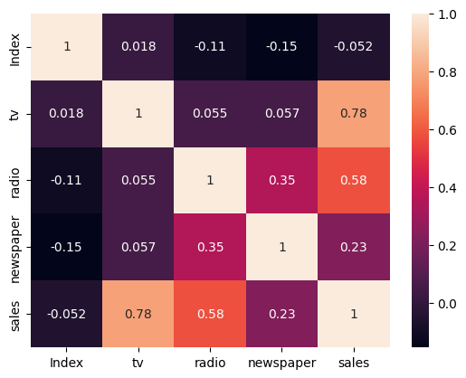
sns.heatmap(advertising.corr(), annot=True)
<Axes: >
from scipy.stats import pearsonr
pearsonr(advertising['tv'],advertising['radio'])
PearsonRResult(statistic=0.05480866446583009, pvalue=0.440806063788431)
The correlation between tv and radio is not statistically significant.
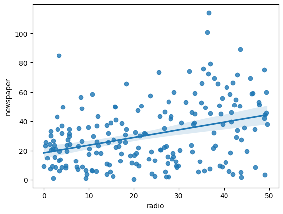
pearsonr(advertising['newspaper'],advertising['radio'])
PearsonRResult(statistic=0.35410375076117534, pvalue=2.688835078719109e-07)
from statsmodels.formula.api import ols
ols("newspaper ~ radio", advertising).fit().summary().tables[1]
| coef | std err | t | P>|t| | [0.025 | 0.975] | |
|---|---|---|---|---|---|---|
| Intercept | 18.4700 | 2.689 | 6.870 | 0.000 | 13.168 | 23.772 |
| radio | 0.5194 | 0.097 | 5.328 | 0.000 | 0.327 | 0.712 |
ols("radio ~ newspaper", advertising).fit().summary().tables[1]
| coef | std err | t | P>|t| | [0.025 | 0.975] | |
|---|---|---|---|---|---|---|
| Intercept | 15.8883 | 1.699 | 9.354 | 0.000 | 12.539 | 19.238 |
| newspaper | 0.2414 | 0.045 | 5.328 | 0.000 | 0.152 | 0.331 |
sns.regplot(x='radio', y='newspaper', data=advertising)
<Axes: xlabel='radio', ylabel='newspaper'>
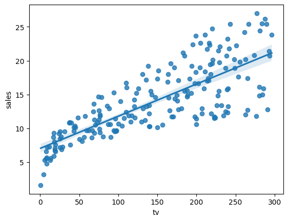
ols("sales ~ tv", advertising).fit().summary()
| Dep. Variable: | sales | R-squared: | 0.612 |
|---|---|---|---|
| Model: | OLS | Adj. R-squared: | 0.610 |
| Method: | Least Squares | F-statistic: | 312.1 |
| Date: | Thu, 30 Nov 2023 | Prob (F-statistic): | 1.47e-42 |
| Time: | 19:48:09 | Log-Likelihood: | -519.05 |
| No. Observations: | 200 | AIC: | 1042. |
| Df Residuals: | 198 | BIC: | 1049. |
| Df Model: | 1 | ||
| Covariance Type: | nonrobust |
| coef | std err | t | P>|t| | [0.025 | 0.975] | |
|---|---|---|---|---|---|---|
| Intercept | 7.0326 | 0.458 | 15.360 | 0.000 | 6.130 | 7.935 |
| tv | 0.0475 | 0.003 | 17.668 | 0.000 | 0.042 | 0.053 |
| Omnibus: | 0.531 | Durbin-Watson: | 1.935 |
|---|---|---|---|
| Prob(Omnibus): | 0.767 | Jarque-Bera (JB): | 0.669 |
| Skew: | -0.089 | Prob(JB): | 0.716 |
| Kurtosis: | 2.779 | Cond. No. | 338. |
Notes:
[1] Standard Errors assume that the covariance matrix of the errors is correctly specified.
sns.regplot(x='tv', y='sales', data=advertising)
<Axes: xlabel='tv', ylabel='sales'>
import statsmodels.api as sm
from matplotlib import pyplot as plt
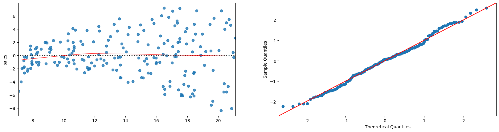
model=ols("sales ~ tv", advertising).fit()
#otteniamo i valori predetti dal modello:
fitted = model.fittedvalues.fillna(0) #rimpiazzo eventuali NaN con zero
plt.figure(figsize=(20,22))
sns.residplot(x=fitted, y='sales', data=advertising.dropna(),lowess=True,line_kws={'color': 'red', 'lw': 1, 'alpha': 0.8}, ax=plt.subplot(421))
sm.qqplot(fitted-advertising.dropna()['sales'], line='45',fit=True, ax=plt.subplot(422))
plt.show()
ols("sales ~ tv + radio", advertising).fit().summary()
| Dep. Variable: | sales | R-squared: | 0.897 |
|---|---|---|---|
| Model: | OLS | Adj. R-squared: | 0.896 |
| Method: | Least Squares | F-statistic: | 859.6 |
| Date: | Thu, 30 Nov 2023 | Prob (F-statistic): | 4.83e-98 |
| Time: | 19:48:42 | Log-Likelihood: | -386.20 |
| No. Observations: | 200 | AIC: | 778.4 |
| Df Residuals: | 197 | BIC: | 788.3 |
| Df Model: | 2 | ||
| Covariance Type: | nonrobust |
| coef | std err | t | P>|t| | [0.025 | 0.975] | |
|---|---|---|---|---|---|---|
| Intercept | 2.9211 | 0.294 | 9.919 | 0.000 | 2.340 | 3.502 |
| tv | 0.0458 | 0.001 | 32.909 | 0.000 | 0.043 | 0.048 |
| radio | 0.1880 | 0.008 | 23.382 | 0.000 | 0.172 | 0.204 |
| Omnibus: | 60.022 | Durbin-Watson: | 2.081 |
|---|---|---|---|
| Prob(Omnibus): | 0.000 | Jarque-Bera (JB): | 148.679 |
| Skew: | -1.323 | Prob(JB): | 5.19e-33 |
| Kurtosis: | 6.292 | Cond. No. | 425. |
Notes:
[1] Standard Errors assume that the covariance matrix of the errors is correctly specified.
import statsmodels.api as sm
from matplotlib import pyplot as plt
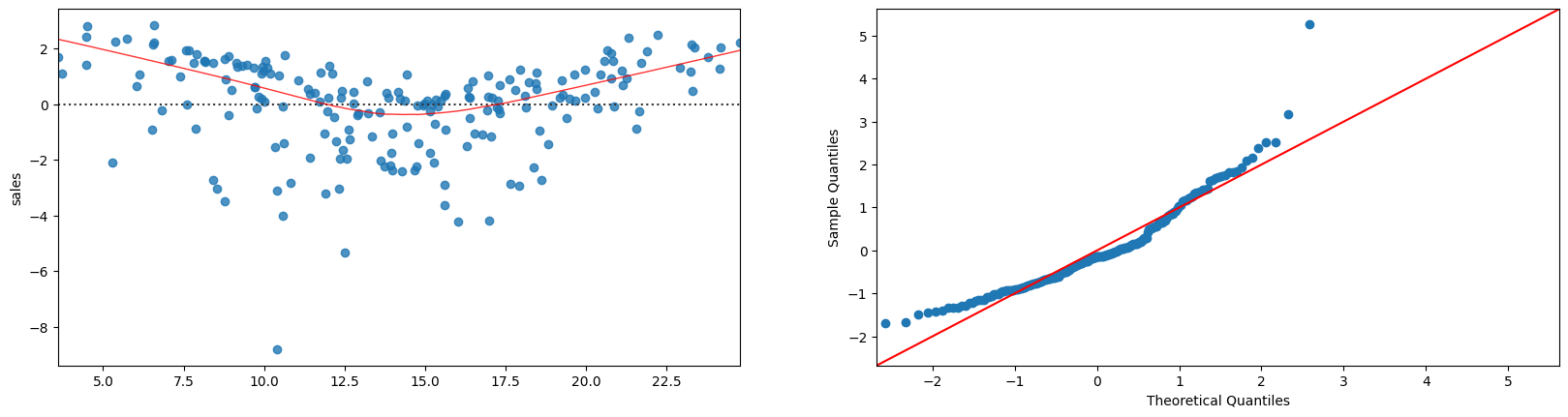
model=ols("sales ~ tv + radio", advertising).fit()
#otteniamo i valori predetti dal modello:
fitted = model.fittedvalues.fillna(0) #rimpiazzo eventuali NaN con zero
plt.figure(figsize=(20,22))
sns.residplot(x=fitted, y='sales', data=advertising.dropna(),lowess=True,line_kws={'color': 'red', 'lw': 1, 'alpha': 0.8}, ax=plt.subplot(421))
sm.qqplot(fitted-advertising.dropna()['sales'], line='45',fit=True, ax=plt.subplot(422))
plt.show()
Let us add an interaction term:
ols("sales ~ tv + radio + radio*tv", advertising).fit().summary()
| Dep. Variable: | sales | R-squared: | 0.968 |
|---|---|---|---|
| Model: | OLS | Adj. R-squared: | 0.967 |
| Method: | Least Squares | F-statistic: | 1963. |
| Date: | Thu, 30 Nov 2023 | Prob (F-statistic): | 6.68e-146 |
| Time: | 19:49:14 | Log-Likelihood: | -270.14 |
| No. Observations: | 200 | AIC: | 548.3 |
| Df Residuals: | 196 | BIC: | 561.5 |
| Df Model: | 3 | ||
| Covariance Type: | nonrobust |
| coef | std err | t | P>|t| | [0.025 | 0.975] | |
|---|---|---|---|---|---|---|
| Intercept | 6.7502 | 0.248 | 27.233 | 0.000 | 6.261 | 7.239 |
| tv | 0.0191 | 0.002 | 12.699 | 0.000 | 0.016 | 0.022 |
| radio | 0.0289 | 0.009 | 3.241 | 0.001 | 0.011 | 0.046 |
| radio:tv | 0.0011 | 5.24e-05 | 20.727 | 0.000 | 0.001 | 0.001 |
| Omnibus: | 128.132 | Durbin-Watson: | 2.224 |
|---|---|---|---|
| Prob(Omnibus): | 0.000 | Jarque-Bera (JB): | 1183.719 |
| Skew: | -2.323 | Prob(JB): | 9.09e-258 |
| Kurtosis: | 13.975 | Cond. No. | 1.80e+04 |
Notes:
[1] Standard Errors assume that the covariance matrix of the errors is correctly specified.
[2] The condition number is large, 1.8e+04. This might indicate that there are
strong multicollinearity or other numerical problems.
The regressor with interaction terms can be interpreted as follows:
33.2. Linear Regression vs Mean Values#
import numpy as np
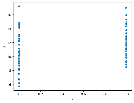
x = np.random.normal(0,2,100)>0
y = np.random.normal(10,2,100) + 2*x
d= pd.DataFrame({
'y': y,
'x': x
})
d['x']=d['x'].astype(int)
d
| y | x | |
|---|---|---|
| 0 | 10.091945 | 0 |
| 1 | 8.620043 | 1 |
| 2 | 14.530024 | 0 |
| 3 | 16.894454 | 1 |
| 4 | 10.864606 | 1 |
| ... | ... | ... |
| 95 | 8.241021 | 0 |
| 96 | 7.561387 | 0 |
| 97 | 6.688701 | 0 |
| 98 | 12.406282 | 1 |
| 99 | 8.094310 | 0 |
100 rows × 2 columns
d.describe()
| y | x | |
|---|---|---|
| count | 100.000000 | 100.000000 |
| mean | 11.124978 | 0.490000 |
| std | 2.509474 | 0.502418 |
| min | 5.701657 | 0.000000 |
| 25% | 9.310256 | 0.000000 |
| 50% | 10.770151 | 0.000000 |
| 75% | 12.717417 | 1.000000 |
| max | 17.218798 | 1.000000 |
d[d['x']==0]['y'].mean()
10.18727989115969
d[d['x']==1]['y'].mean()
12.100950474439491
d[d['x']==0]['y'].mean() + 2.2391
12.42637989115969
ols('y ~ x', d).fit().summary()
| Dep. Variable: | y | R-squared: | 0.147 |
|---|---|---|---|
| Model: | OLS | Adj. R-squared: | 0.138 |
| Method: | Least Squares | F-statistic: | 16.86 |
| Date: | Thu, 30 Nov 2023 | Prob (F-statistic): | 8.34e-05 |
| Time: | 19:50:08 | Log-Likelihood: | -225.46 |
| No. Observations: | 100 | AIC: | 454.9 |
| Df Residuals: | 98 | BIC: | 460.1 |
| Df Model: | 1 | ||
| Covariance Type: | nonrobust |
| coef | std err | t | P>|t| | [0.025 | 0.975] | |
|---|---|---|---|---|---|---|
| Intercept | 10.1873 | 0.326 | 31.227 | 0.000 | 9.540 | 10.835 |
| x | 1.9137 | 0.466 | 4.106 | 0.000 | 0.989 | 2.839 |
| Omnibus: | 3.658 | Durbin-Watson: | 2.063 |
|---|---|---|---|
| Prob(Omnibus): | 0.161 | Jarque-Bera (JB): | 3.568 |
| Skew: | 0.458 | Prob(JB): | 0.168 |
| Kurtosis: | 2.863 | Cond. No. | 2.60 |
Notes:
[1] Standard Errors assume that the covariance matrix of the errors is correctly specified.
sns.scatterplot(x='x', y='y', data=d)
<Axes: xlabel='x', ylabel='y'>
33.3. Logistic regression#
We will consider this dataset:
https://www.kaggle.com/datasets/redwankarimsony/heart-disease-data
data=pd.read_csv('heart_disease_uci.csv')
data.head()
| id | age | sex | dataset | cp | trestbps | chol | fbs | restecg | thalch | exang | oldpeak | slope | ca | thal | num | |
|---|---|---|---|---|---|---|---|---|---|---|---|---|---|---|---|---|
| 0 | 1 | 63 | Male | Cleveland | typical angina | 145.0 | 233.0 | True | lv hypertrophy | 150.0 | False | 2.3 | downsloping | 0.0 | fixed defect | 0 |
| 1 | 2 | 67 | Male | Cleveland | asymptomatic | 160.0 | 286.0 | False | lv hypertrophy | 108.0 | True | 1.5 | flat | 3.0 | normal | 2 |
| 2 | 3 | 67 | Male | Cleveland | asymptomatic | 120.0 | 229.0 | False | lv hypertrophy | 129.0 | True | 2.6 | flat | 2.0 | reversable defect | 1 |
| 3 | 4 | 37 | Male | Cleveland | non-anginal | 130.0 | 250.0 | False | normal | 187.0 | False | 3.5 | downsloping | 0.0 | normal | 0 |
| 4 | 5 | 41 | Female | Cleveland | atypical angina | 130.0 | 204.0 | False | lv hypertrophy | 172.0 | False | 1.4 | upsloping | 0.0 | normal | 0 |
data['attack'] = (data['num']>0).astype(int)
data.describe()
| id | age | trestbps | chol | thalch | oldpeak | ca | num | attack | |
|---|---|---|---|---|---|---|---|---|---|
| count | 920.000000 | 920.000000 | 861.000000 | 890.000000 | 865.000000 | 858.000000 | 309.000000 | 920.000000 | 920.000000 |
| mean | 460.500000 | 53.510870 | 132.132404 | 199.130337 | 137.545665 | 0.878788 | 0.676375 | 0.995652 | 0.553261 |
| std | 265.725422 | 9.424685 | 19.066070 | 110.780810 | 25.926276 | 1.091226 | 0.935653 | 1.142693 | 0.497426 |
| min | 1.000000 | 28.000000 | 0.000000 | 0.000000 | 60.000000 | -2.600000 | 0.000000 | 0.000000 | 0.000000 |
| 25% | 230.750000 | 47.000000 | 120.000000 | 175.000000 | 120.000000 | 0.000000 | 0.000000 | 0.000000 | 0.000000 |
| 50% | 460.500000 | 54.000000 | 130.000000 | 223.000000 | 140.000000 | 0.500000 | 0.000000 | 1.000000 | 1.000000 |
| 75% | 690.250000 | 60.000000 | 140.000000 | 268.000000 | 157.000000 | 1.500000 | 1.000000 | 2.000000 | 1.000000 |
| max | 920.000000 | 77.000000 | 200.000000 | 603.000000 | 202.000000 | 6.200000 | 3.000000 | 4.000000 | 1.000000 |
from statsmodels.formula.api import logit
logit("attack ~ sex", data).fit().summary()
Optimization terminated successfully.
         Current function value: 0.639394
         Iterations 5
| Dep. Variable: | attack | No. Observations: | 920 |
|---|---|---|---|
| Model: | Logit | Df Residuals: | 918 |
| Method: | MLE | Df Model: | 1 |
| Date: | Thu, 30 Nov 2023 | Pseudo R-squ.: | 0.06992 |
| Time: | 19:51:22 | Log-Likelihood: | -588.24 |
| converged: | True | LL-Null: | -632.47 |
| Covariance Type: | nonrobust | LLR p-value: | 5.220e-21 |
| coef | std err | z | P>|z| | [0.025 | 0.975] | |
|---|---|---|---|---|---|---|
| Intercept | -1.0578 | 0.164 | -6.444 | 0.000 | -1.380 | -0.736 |
| sex[T.Male] | 1.5996 | 0.181 | 8.823 | 0.000 | 1.244 | 1.955 |
The coefficient of sex[T.Male] is telling us that males have a risk of heart attack \(e^{1.5996} \approx 4.95\) times higher than females.
To compute a multiple logistic regressor, let us first extend the dataset with dummy variables:
data2 = pd.get_dummies(data.dropna(), columns=["sex", "dataset", "cp", "fbs", "restecg", "exang", "slope", "thal"], drop_first=True)
We will use the non-forumla API:
from statsmodels.api import Logit
data2['Intercept']=1 # we need to add the intercept manually when using this API
Logit(data2['attack'], data2.drop(['dataset','attack','num','id'],axis=1)).fit().summary()
Optimization terminated successfully.
         Current function value: 0.321016
         Iterations 8
| Dep. Variable: | attack | No. Observations: | 299 |
|---|---|---|---|
| Model: | Logit | Df Residuals: | 280 |
| Method: | MLE | Df Model: | 18 |
| Date: | Thu, 30 Nov 2023 | Pseudo R-squ.: | 0.5352 |
| Time: | 20:04:07 | Log-Likelihood: | -95.984 |
| converged: | True | LL-Null: | -206.51 |
| Covariance Type: | nonrobust | LLR p-value: | 5.920e-37 |
| coef | std err | z | P>|z| | [0.025 | 0.975] | |
|---|---|---|---|---|---|---|
| age | -0.0137 | 0.025 | -0.554 | 0.579 | -0.062 | 0.035 |
| trestbps | 0.0244 | 0.011 | 2.170 | 0.030 | 0.002 | 0.046 |
| chol | 0.0042 | 0.004 | 1.064 | 0.287 | -0.004 | 0.012 |
| thalch | -0.0180 | 0.011 | -1.625 | 0.104 | -0.040 | 0.004 |
| oldpeak | 0.3610 | 0.231 | 1.566 | 0.117 | -0.091 | 0.813 |
| ca | 1.3099 | 0.280 | 4.682 | 0.000 | 0.762 | 1.858 |
| sex_Male | 1.5500 | 0.531 | 2.920 | 0.003 | 0.510 | 2.590 |
| cp_atypical angina | -0.8454 | 0.561 | -1.508 | 0.132 | -1.944 | 0.253 |
| cp_non-anginal | -1.8501 | 0.501 | -3.690 | 0.000 | -2.833 | -0.867 |
| cp_typical angina | -2.1010 | 0.667 | -3.151 | 0.002 | -3.408 | -0.794 |
| fbs_True | -0.5952 | 0.609 | -0.977 | 0.329 | -1.789 | 0.599 |
| restecg_normal | -0.4695 | 0.384 | -1.222 | 0.222 | -1.222 | 0.283 |
| restecg_st-t abnormality | 0.3128 | 2.439 | 0.128 | 0.898 | -4.467 | 5.092 |
| exang_True | 0.7190 | 0.440 | 1.634 | 0.102 | -0.143 | 1.581 |
| slope_flat | 0.6474 | 0.851 | 0.761 | 0.447 | -1.020 | 2.315 |
| slope_upsloping | -0.5167 | 0.922 | -0.560 | 0.575 | -2.325 | 1.291 |
| thal_normal | 0.0313 | 0.790 | 0.040 | 0.968 | -1.517 | 1.579 |
| thal_reversable defect | 1.4329 | 0.775 | 1.850 | 0.064 | -0.085 | 2.951 |
| Intercept | -2.8907 | 2.847 | -1.015 | 0.310 | -8.472 | 2.690 |
Let us proceed removing the variables with largest p-values wih backward elimination. We’ll drop thal_normal:
Logit(data2['attack'], data2.drop(['dataset','attack','num','id','thal_normal'],axis=1)).fit().summary()
Optimization terminated successfully.
         Current function value: 0.321018
         Iterations 8
| Dep. Variable: | attack | No. Observations: | 299 |
|---|---|---|---|
| Model: | Logit | Df Residuals: | 281 |
| Method: | MLE | Df Model: | 17 |
| Date: | Thu, 30 Nov 2023 | Pseudo R-squ.: | 0.5352 |
| Time: | 20:05:21 | Log-Likelihood: | -95.984 |
| converged: | True | LL-Null: | -206.51 |
| Covariance Type: | nonrobust | LLR p-value: | 1.611e-37 |
| coef | std err | z | P>|z| | [0.025 | 0.975] | |
|---|---|---|---|---|---|---|
| age | -0.0137 | 0.025 | -0.555 | 0.579 | -0.062 | 0.035 |
| trestbps | 0.0244 | 0.011 | 2.171 | 0.030 | 0.002 | 0.046 |
| chol | 0.0042 | 0.004 | 1.067 | 0.286 | -0.004 | 0.012 |
| thalch | -0.0180 | 0.011 | -1.636 | 0.102 | -0.040 | 0.004 |
| oldpeak | 0.3604 | 0.230 | 1.567 | 0.117 | -0.090 | 0.811 |
| ca | 1.3098 | 0.280 | 4.682 | 0.000 | 0.761 | 1.858 |
| sex_Male | 1.5445 | 0.512 | 3.016 | 0.003 | 0.541 | 2.548 |
| cp_atypical angina | -0.8443 | 0.560 | -1.508 | 0.132 | -1.942 | 0.253 |
| cp_non-anginal | -1.8479 | 0.498 | -3.709 | 0.000 | -2.824 | -0.871 |
| cp_typical angina | -2.0968 | 0.658 | -3.186 | 0.001 | -3.387 | -0.807 |
| fbs_True | -0.5979 | 0.605 | -0.988 | 0.323 | -1.784 | 0.589 |
| restecg_normal | -0.4707 | 0.383 | -1.229 | 0.219 | -1.221 | 0.280 |
| restecg_st-t abnormality | 0.3147 | 2.439 | 0.129 | 0.897 | -4.465 | 5.094 |
| exang_True | 0.7186 | 0.440 | 1.634 | 0.102 | -0.143 | 1.581 |
| slope_flat | 0.6484 | 0.850 | 0.763 | 0.446 | -1.018 | 2.314 |
| slope_upsloping | -0.5133 | 0.919 | -0.559 | 0.576 | -2.314 | 1.287 |
| thal_reversable defect | 1.4068 | 0.405 | 3.471 | 0.001 | 0.612 | 2.201 |
| Intercept | -2.8676 | 2.786 | -1.029 | 0.303 | -8.329 | 2.593 |
Let us remove restecg_st-t abnormality:
Logit(data2['attack'], data2.drop(['dataset','attack','num','id','restecg_st-t abnormality','thal_normal'],axis=1)).fit().summary()
Optimization terminated successfully.
         Current function value: 0.321046
         Iterations 7
| Dep. Variable: | attack | No. Observations: | 299 |
|---|---|---|---|
| Model: | Logit | Df Residuals: | 282 |
| Method: | MLE | Df Model: | 16 |
| Date: | Thu, 30 Nov 2023 | Pseudo R-squ.: | 0.5352 |
| Time: | 20:05:33 | Log-Likelihood: | -95.993 |
| converged: | True | LL-Null: | -206.51 |
| Covariance Type: | nonrobust | LLR p-value: | 4.281e-38 |
| coef | std err | z | P>|z| | [0.025 | 0.975] | |
|---|---|---|---|---|---|---|
| age | -0.0137 | 0.025 | -0.553 | 0.581 | -0.062 | 0.035 |
| trestbps | 0.0245 | 0.011 | 2.187 | 0.029 | 0.003 | 0.046 |
| chol | 0.0042 | 0.004 | 1.061 | 0.289 | -0.004 | 0.012 |
| thalch | -0.0181 | 0.011 | -1.650 | 0.099 | -0.040 | 0.003 |
| oldpeak | 0.3633 | 0.229 | 1.588 | 0.112 | -0.085 | 0.812 |
| ca | 1.3091 | 0.280 | 4.680 | 0.000 | 0.761 | 1.857 |
| sex_Male | 1.5371 | 0.508 | 3.023 | 0.003 | 0.541 | 2.534 |
| cp_atypical angina | -0.8440 | 0.560 | -1.507 | 0.132 | -1.942 | 0.254 |
| cp_non-anginal | -1.8463 | 0.498 | -3.705 | 0.000 | -2.823 | -0.870 |
| cp_typical angina | -2.0996 | 0.658 | -3.192 | 0.001 | -3.389 | -0.810 |
| fbs_True | -0.6002 | 0.605 | -0.991 | 0.321 | -1.787 | 0.586 |
| restecg_normal | -0.4752 | 0.381 | -1.246 | 0.213 | -1.223 | 0.272 |
| exang_True | 0.7188 | 0.440 | 1.634 | 0.102 | -0.143 | 1.581 |
| slope_flat | 0.6525 | 0.850 | 0.768 | 0.443 | -1.014 | 2.319 |
| slope_upsloping | -0.5079 | 0.918 | -0.553 | 0.580 | -2.308 | 1.292 |
| thal_reversable defect | 1.4075 | 0.405 | 3.474 | 0.001 | 0.614 | 2.202 |
| Intercept | -2.8552 | 2.784 | -1.025 | 0.305 | -8.312 | 2.602 |
We now remove age:
Logit(data2['attack'], data2.drop(['dataset','attack','num','id','restecg_st-t abnormality','thal_normal','age'],axis=1)).fit().summary()
Optimization terminated successfully.
         Current function value: 0.321559
         Iterations 7
| Dep. Variable: | attack | No. Observations: | 299 |
|---|---|---|---|
| Model: | Logit | Df Residuals: | 283 |
| Method: | MLE | Df Model: | 15 |
| Date: | Thu, 30 Nov 2023 | Pseudo R-squ.: | 0.5344 |
| Time: | 20:05:46 | Log-Likelihood: | -96.146 |
| converged: | True | LL-Null: | -206.51 |
| Covariance Type: | nonrobust | LLR p-value: | 1.261e-38 |
| coef | std err | z | P>|z| | [0.025 | 0.975] | |
|---|---|---|---|---|---|---|
| trestbps | 0.0228 | 0.011 | 2.126 | 0.034 | 0.002 | 0.044 |
| chol | 0.0039 | 0.004 | 1.002 | 0.316 | -0.004 | 0.011 |
| thalch | -0.0159 | 0.010 | -1.561 | 0.119 | -0.036 | 0.004 |
| oldpeak | 0.3710 | 0.228 | 1.626 | 0.104 | -0.076 | 0.818 |
| ca | 1.2705 | 0.269 | 4.718 | 0.000 | 0.743 | 1.798 |
| sex_Male | 1.5667 | 0.504 | 3.106 | 0.002 | 0.578 | 2.555 |
| cp_atypical angina | -0.8593 | 0.560 | -1.536 | 0.125 | -1.956 | 0.237 |
| cp_non-anginal | -1.8614 | 0.498 | -3.738 | 0.000 | -2.837 | -0.885 |
| cp_typical angina | -2.1148 | 0.656 | -3.224 | 0.001 | -3.400 | -0.829 |
| fbs_True | -0.6053 | 0.602 | -1.006 | 0.315 | -1.785 | 0.574 |
| restecg_normal | -0.4670 | 0.381 | -1.227 | 0.220 | -1.213 | 0.279 |
| exang_True | 0.7299 | 0.438 | 1.666 | 0.096 | -0.129 | 1.589 |
| slope_flat | 0.6455 | 0.851 | 0.758 | 0.448 | -1.023 | 2.314 |
| slope_upsloping | -0.5038 | 0.920 | -0.548 | 0.584 | -2.307 | 1.299 |
| thal_reversable defect | 1.3990 | 0.404 | 3.466 | 0.001 | 0.608 | 2.190 |
| Intercept | -3.6527 | 2.381 | -1.534 | 0.125 | -8.319 | 1.013 |
It’s now the turn of slope_upsloping:
Logit(data2['attack'], data2.drop(['dataset','attack','num','id','restecg_st-t abnormality','thal_normal','age','slope_upsloping'],axis=1)).fit().summary()
Optimization terminated successfully.
         Current function value: 0.322049
         Iterations 7
| Dep. Variable: | attack | No. Observations: | 299 |
|---|---|---|---|
| Model: | Logit | Df Residuals: | 284 |
| Method: | MLE | Df Model: | 14 |
| Date: | Thu, 30 Nov 2023 | Pseudo R-squ.: | 0.5337 |
| Time: | 20:05:54 | Log-Likelihood: | -96.293 |
| converged: | True | LL-Null: | -206.51 |
| Covariance Type: | nonrobust | LLR p-value: | 3.566e-39 |
| coef | std err | z | P>|z| | [0.025 | 0.975] | |
|---|---|---|---|---|---|---|
| trestbps | 0.0227 | 0.011 | 2.116 | 0.034 | 0.002 | 0.044 |
| chol | 0.0037 | 0.004 | 0.970 | 0.332 | -0.004 | 0.011 |
| thalch | -0.0164 | 0.010 | -1.619 | 0.105 | -0.036 | 0.003 |
| oldpeak | 0.4256 | 0.205 | 2.078 | 0.038 | 0.024 | 0.827 |
| ca | 1.2458 | 0.264 | 4.715 | 0.000 | 0.728 | 1.764 |
| sex_Male | 1.5501 | 0.502 | 3.087 | 0.002 | 0.566 | 2.534 |
| cp_atypical angina | -0.8492 | 0.558 | -1.521 | 0.128 | -1.943 | 0.245 |
| cp_non-anginal | -1.8661 | 0.498 | -3.744 | 0.000 | -2.843 | -0.889 |
| cp_typical angina | -2.1161 | 0.654 | -3.235 | 0.001 | -3.398 | -0.834 |
| fbs_True | -0.5632 | 0.594 | -0.947 | 0.343 | -1.728 | 0.602 |
| restecg_normal | -0.4814 | 0.379 | -1.269 | 0.205 | -1.225 | 0.262 |
| exang_True | 0.7304 | 0.438 | 1.669 | 0.095 | -0.127 | 1.588 |
| slope_flat | 1.0485 | 0.429 | 2.442 | 0.015 | 0.207 | 1.890 |
| thal_reversable defect | 1.4014 | 0.404 | 3.472 | 0.001 | 0.610 | 2.193 |
| Intercept | -3.9750 | 2.302 | -1.727 | 0.084 | -8.487 | 0.537 |
Let’s remove fbs_True:
Logit(data2['attack'], data2.drop(['dataset','attack','num','id','restecg_st-t abnormality','thal_normal','age','slope_upsloping','fbs_True'],axis=1)).fit().summary()
Optimization terminated successfully.
         Current function value: 0.323582
         Iterations 7
| Dep. Variable: | attack | No. Observations: | 299 |
|---|---|---|---|
| Model: | Logit | Df Residuals: | 285 |
| Method: | MLE | Df Model: | 13 |
| Date: | Thu, 30 Nov 2023 | Pseudo R-squ.: | 0.5315 |
| Time: | 20:06:06 | Log-Likelihood: | -96.751 |
| converged: | True | LL-Null: | -206.51 |
| Covariance Type: | nonrobust | LLR p-value: | 1.307e-39 |
| coef | std err | z | P>|z| | [0.025 | 0.975] | |
|---|---|---|---|---|---|---|
| trestbps | 0.0210 | 0.011 | 1.998 | 0.046 | 0.000 | 0.042 |
| chol | 0.0036 | 0.004 | 0.936 | 0.349 | -0.004 | 0.011 |
| thalch | -0.0164 | 0.010 | -1.628 | 0.103 | -0.036 | 0.003 |
| oldpeak | 0.4380 | 0.205 | 2.135 | 0.033 | 0.036 | 0.840 |
| ca | 1.1942 | 0.256 | 4.664 | 0.000 | 0.692 | 1.696 |
| sex_Male | 1.4928 | 0.498 | 3.000 | 0.003 | 0.518 | 2.468 |
| cp_atypical angina | -0.8841 | 0.554 | -1.596 | 0.110 | -1.970 | 0.201 |
| cp_non-anginal | -1.9746 | 0.489 | -4.039 | 0.000 | -2.933 | -1.016 |
| cp_typical angina | -2.1802 | 0.653 | -3.340 | 0.001 | -3.460 | -0.901 |
| restecg_normal | -0.4735 | 0.379 | -1.250 | 0.211 | -1.216 | 0.269 |
| exang_True | 0.6861 | 0.435 | 1.578 | 0.115 | -0.166 | 1.539 |
| slope_flat | 1.0228 | 0.428 | 2.391 | 0.017 | 0.184 | 1.861 |
| thal_reversable defect | 1.4331 | 0.402 | 3.564 | 0.000 | 0.645 | 2.221 |
| Intercept | -3.6750 | 2.257 | -1.628 | 0.104 | -8.099 | 0.749 |
Let’s remove chol:
Logit(data2['attack'], data2.drop(['dataset','attack','num','id','restecg_st-t abnormality','thal_normal','age','slope_upsloping','fbs_True','chol'],axis=1)).fit().summary()
Optimization terminated successfully.
         Current function value: 0.325012
         Iterations 7
| Dep. Variable: | attack | No. Observations: | 299 |
|---|---|---|---|
| Model: | Logit | Df Residuals: | 286 |
| Method: | MLE | Df Model: | 12 |
| Date: | Thu, 30 Nov 2023 | Pseudo R-squ.: | 0.5294 |
| Time: | 20:06:19 | Log-Likelihood: | -97.179 |
| converged: | True | LL-Null: | -206.51 |
| Covariance Type: | nonrobust | LLR p-value: | 4.481e-40 |
| coef | std err | z | P>|z| | [0.025 | 0.975] | |
|---|---|---|---|---|---|---|
| trestbps | 0.0215 | 0.010 | 2.045 | 0.041 | 0.001 | 0.042 |
| thalch | -0.0152 | 0.010 | -1.538 | 0.124 | -0.035 | 0.004 |
| oldpeak | 0.4460 | 0.205 | 2.174 | 0.030 | 0.044 | 0.848 |
| ca | 1.1928 | 0.255 | 4.686 | 0.000 | 0.694 | 1.692 |
| sex_Male | 1.3485 | 0.467 | 2.889 | 0.004 | 0.434 | 2.263 |
| cp_atypical angina | -0.8627 | 0.551 | -1.565 | 0.118 | -1.943 | 0.218 |
| cp_non-anginal | -1.9666 | 0.488 | -4.026 | 0.000 | -2.924 | -1.009 |
| cp_typical angina | -2.1905 | 0.651 | -3.365 | 0.001 | -3.466 | -0.915 |
| restecg_normal | -0.5380 | 0.371 | -1.448 | 0.147 | -1.266 | 0.190 |
| exang_True | 0.6821 | 0.432 | 1.579 | 0.114 | -0.164 | 1.529 |
| slope_flat | 1.0435 | 0.427 | 2.446 | 0.014 | 0.207 | 1.880 |
| thal_reversable defect | 1.4706 | 0.402 | 3.659 | 0.000 | 0.683 | 2.258 |
| Intercept | -2.9396 | 2.092 | -1.405 | 0.160 | -7.039 | 1.160 |
Let’s remove restecg_normal:
Logit(data2['attack'], data2.drop(['dataset','attack','num','id','restecg_st-t abnormality','thal_normal','age','slope_upsloping','fbs_True','chol','restecg_normal'],axis=1)).fit().summary()
Optimization terminated successfully.
         Current function value: 0.328559
         Iterations 7
| Dep. Variable: | attack | No. Observations: | 299 |
|---|---|---|---|
| Model: | Logit | Df Residuals: | 287 |
| Method: | MLE | Df Model: | 11 |
| Date: | Thu, 30 Nov 2023 | Pseudo R-squ.: | 0.5243 |
| Time: | 20:06:47 | Log-Likelihood: | -98.239 |
| converged: | True | LL-Null: | -206.51 |
| Covariance Type: | nonrobust | LLR p-value: | 2.704e-40 |
| coef | std err | z | P>|z| | [0.025 | 0.975] | |
|---|---|---|---|---|---|---|
| trestbps | 0.0225 | 0.010 | 2.196 | 0.028 | 0.002 | 0.043 |
| thalch | -0.0152 | 0.010 | -1.530 | 0.126 | -0.035 | 0.004 |
| oldpeak | 0.4357 | 0.200 | 2.183 | 0.029 | 0.045 | 0.827 |
| ca | 1.2152 | 0.253 | 4.806 | 0.000 | 0.720 | 1.711 |
| sex_Male | 1.3796 | 0.466 | 2.961 | 0.003 | 0.466 | 2.293 |
| cp_atypical angina | -0.8622 | 0.550 | -1.567 | 0.117 | -1.940 | 0.216 |
| cp_non-anginal | -1.9589 | 0.485 | -4.038 | 0.000 | -2.910 | -1.008 |
| cp_typical angina | -2.1394 | 0.646 | -3.313 | 0.001 | -3.405 | -0.874 |
| exang_True | 0.6737 | 0.432 | 1.560 | 0.119 | -0.173 | 1.520 |
| slope_flat | 1.1014 | 0.422 | 2.608 | 0.009 | 0.274 | 1.929 |
| thal_reversable defect | 1.4078 | 0.395 | 3.567 | 0.000 | 0.634 | 2.181 |
| Intercept | -3.3894 | 2.056 | -1.648 | 0.099 | -7.420 | 0.641 |
Let us now remove exang_True:
Logit(data2['attack'], data2.drop(['dataset','attack','num','id','restecg_st-t abnormality','thal_normal','age','slope_upsloping','fbs_True','chol','restecg_normal','exang_True'],axis=1)).fit().summary()
Optimization terminated successfully.
         Current function value: 0.332571
         Iterations 7
| Dep. Variable: | attack | No. Observations: | 299 |
|---|---|---|---|
| Model: | Logit | Df Residuals: | 288 |
| Method: | MLE | Df Model: | 10 |
| Date: | Thu, 30 Nov 2023 | Pseudo R-squ.: | 0.5185 |
| Time: | 20:07:11 | Log-Likelihood: | -99.439 |
| converged: | True | LL-Null: | -206.51 |
| Covariance Type: | nonrobust | LLR p-value: | 1.791e-40 |
| coef | std err | z | P>|z| | [0.025 | 0.975] | |
|---|---|---|---|---|---|---|
| trestbps | 0.0233 | 0.010 | 2.278 | 0.023 | 0.003 | 0.043 |
| thalch | -0.0180 | 0.010 | -1.845 | 0.065 | -0.037 | 0.001 |
| oldpeak | 0.4647 | 0.197 | 2.354 | 0.019 | 0.078 | 0.852 |
| ca | 1.2033 | 0.252 | 4.781 | 0.000 | 0.710 | 1.697 |
| sex_Male | 1.3780 | 0.458 | 3.006 | 0.003 | 0.480 | 2.276 |
| cp_atypical angina | -1.0592 | 0.537 | -1.973 | 0.048 | -2.111 | -0.007 |
| cp_non-anginal | -2.1451 | 0.472 | -4.549 | 0.000 | -3.069 | -1.221 |
| cp_typical angina | -2.3297 | 0.642 | -3.626 | 0.000 | -3.589 | -1.071 |
| slope_flat | 1.1436 | 0.420 | 2.724 | 0.006 | 0.321 | 1.966 |
| thal_reversable defect | 1.4692 | 0.391 | 3.758 | 0.000 | 0.703 | 2.235 |
| Intercept | -2.8221 | 2.011 | -1.404 | 0.160 | -6.763 | 1.119 |
Let us now remove thalch:
Logit(data2['attack'], data2.drop(['dataset','attack','num','id','restecg_st-t abnormality','thal_normal','age','slope_upsloping','fbs_True','chol','restecg_normal','exang_True','thalch'],axis=1)).fit().summary()
Optimization terminated successfully.
         Current function value: 0.338536
         Iterations 7
| Dep. Variable: | attack | No. Observations: | 299 |
|---|---|---|---|
| Model: | Logit | Df Residuals: | 289 |
| Method: | MLE | Df Model: | 9 |
| Date: | Thu, 30 Nov 2023 | Pseudo R-squ.: | 0.5099 |
| Time: | 20:07:42 | Log-Likelihood: | -101.22 |
| converged: | True | LL-Null: | -206.51 |
| Covariance Type: | nonrobust | LLR p-value: | 1.996e-40 |
| coef | std err | z | P>|z| | [0.025 | 0.975] | |
|---|---|---|---|---|---|---|
| trestbps | 0.0220 | 0.010 | 2.145 | 0.032 | 0.002 | 0.042 |
| oldpeak | 0.5145 | 0.194 | 2.659 | 0.008 | 0.135 | 0.894 |
| ca | 1.2539 | 0.252 | 4.985 | 0.000 | 0.761 | 1.747 |
| sex_Male | 1.3382 | 0.455 | 2.942 | 0.003 | 0.447 | 2.230 |
| cp_atypical angina | -1.2521 | 0.521 | -2.403 | 0.016 | -2.274 | -0.231 |
| cp_non-anginal | -2.3023 | 0.464 | -4.966 | 0.000 | -3.211 | -1.394 |
| cp_typical angina | -2.5791 | 0.644 | -4.004 | 0.000 | -3.842 | -1.317 |
| slope_flat | 1.3792 | 0.397 | 3.470 | 0.001 | 0.600 | 2.158 |
| thal_reversable defect | 1.5143 | 0.388 | 3.907 | 0.000 | 0.755 | 2.274 |
| Intercept | -5.4495 | 1.485 | -3.669 | 0.000 | -8.361 | -2.538 |
Al p-values are now below the significance level \(\alpha=0.05\). We can now proceed interpreting the result.