1. Introduction to Data Analysis#
The goal of this first lecture is to give an understanding of what data analysis is. We will initially keep a rather informal tone, while more formal definition will be given later in the course.
Before diving into what Data Analysis is, we need to develop at least an intuitive understanding of what data is, which is addressed in the following sections.
Slides for this section available here.
1.1. What is Data? An informal Definition#
We will start by giving an informal definition of data. It is not by any means a complete definition, but it will suffice as a starting point to get an intuitive understanding of what data is:
Data is a set of values collected with respect to some variables which describe a given phenomenon.
In the definition above, we mentioned some key concepts, which are discussed in the following sections.
1.1.1. Set of Values#
Data is a “set of values”, in the sense that, when we deal with data, we actually deal with multiple instances of values associated to the same event or phenomenon. Examples:
Example |
Comment |
|---|---|
We want to study how the heights of students change with the years |
We need sets of recorded heights, not just one height |
We want to study how a given drug affects the recovering from a disease |
We need to record sets of values about drug assumption and recover, just one case will not be enough |
We need to create a system which can generate text from a prompt |
We need to record several examples of prompt-text generation, just one would not be enough to study how such generation should be made |
Since we deal with sets of values, we will often use the term dataset to refer to a given collection of data related to a given phenomenon.
1.1.2. Data collection#
Data is always collected in some way. This is important to consider, as the collection process may introduce some form of bias or error. While we will get back later on how data can be collected, popular ways to collect data include surveys (asking questions to people) and physical measurements (e.g., physically measuring the heights of people). Note that both collection methods (though these are not the only possible) may bring their own source of error. Indeed, people may lie or report incorrect information, while our measurement tools may be flawed or have a limited precision. In all cases, imperfect data due to the way it has been collected is part of the game (we cannot expert perfect data). We often say that we “observe” data. This is a broader therm to say that we do not come up with data, but it comes from some external source we are interested it (hence we collect it). Hence, we often refer to a given value we deal with as an observation. For instance, the height of a single person in the classroom can be called an observation.
1.1.3. Variables#
The values we collect are associated to abstract entities which we will call “variables”. Again, we will get to a more formal definition later. For the moment, consider that these entities are similar to the mathematical variables we are used to or to the variables we encounter in many programming languages. We could see them as “containers” for the data, but also, and more importantly, as abstract entities defining which data they are expected to hold.
1.1.3.1. Example - Mathematical Variables#
For instance, if we are solving a geometric problem, such as computing the area of a triangle, we may define a variable \(h\) which will be responsible for “containing” the value of the height of the triangle. We can then define a variable \(b\), which will hold the value for the base. We can hence solve the problem of computing the area of the triangle by using the formula
where \(a\) is an additional variable which will “hold” the value of the area. Note that we can observe different triangles and assign different values to each variable every time, but we always expect \(b\) to contain the length of the base, \(h\) to contain the height, and \(a\) to contain the area. If we weren’t to do so, the formula above would be useless.
1.1.3.2. Example - Programming Variables#
Similarly, if we create a computer program to solve the same problem, we will probably define three double variables with the same names and expect them to always contain values coherent with the ones we had in mind when we defined such variabile:
double b;
double h;
double a;

input(&b, &h);

a = (b*h)/2;
1.1.3.3. Example - Statistical Variables#
In a very similar way, when analyzing data, we will define variables expected to contain values related to a specific event or phenomenon. For instance, we may define a statistical variable \(H\) to contain the value of the height of people in the class. We often have more than one variable in a data analysis problem. This is useful when we want to measure or analyze more than one aspect of the problem we are considering. For instance, we may want to measure both the height and weight of people in the class. In that case, we could also introduce an additional statistical variable \(W\) which will contain the values of the weight of people. We may later (as we will see) ask questions on how the values of the two variables are somehow related.
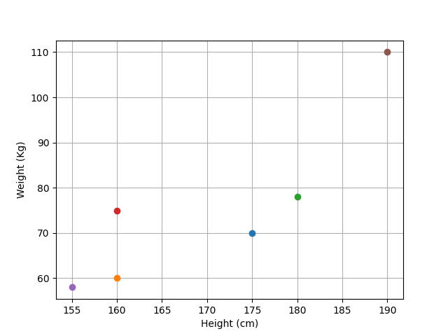
When we have more than one variable related to different aspects of the same event (e.g., height and weight, where the “event” is observing a given person in the classroom), we will say that the set of values related to the given variables is an observation. For instance the pair of values \((H,W)=(175cm, 68Kg)\) can be seen as an observation. Since this pair of values can be represented as a point in a 2D space, we also call it a data point. In this context, a set of observations (e.g., heights and weights of 30 people) is generally called a dataset.
For example, the graph below represents four observations related to the following measurements of six different subjects:
Subject |
Height (cm) |
Weight (Kg) |
|---|---|---|
1 |
175 |
70 |
2 |
160 |
60 |
3 |
180 |
78 |
4 |
160 |
75 |
5 |
155 |
58 |
6 |
190 |
110 |
1.1.4. Phenomenon#
When we analyze data, we are usually interested in investigating some phenomenon. For instance, we may be curious of what is the rate of overweight students in a school. This can be useful, e.g., to understand whether a new diet proposed in the school canteen is generating good or bad consequences. The phenomenon we want to study is important to keep in mind when collecting and analyzing data, as an inappropriate data collection could create some bias or make our conclusions limited. For instance, if we collected only data of male subjects, we may not be able to fully understand the problem we am considering.
1.1.5. An example of a dataset#
Before closing our brief discussion of what data is, it is worth mentioning that datasets are usually stored in tables in which columns represent the different variables and rows represent the different observations. If you have ever had a look at a spreadsheet, you probably already see an example of a dataset!
Let’s conside the following example of a dataset of marks of \(5\) subjects obtained by three students:
Maths |
Geography |
English |
Physics |
Chemistry |
|
|---|---|---|---|---|---|
x001 |
8 |
9 |
30 |
8 |
10 |
x038 |
9 |
7 |
27 |
6 |
|
x002 |
6 |
-1 |
18 |
5 |
6 |
x012 |
7 |
7 |
25 |
4 |
10 |
x042 |
10 |
10 |
30 |
10 |
10 |
Each row is an observation related to a given student, while each column represents a different variable (the marks obtained in the different courses).
Before moving on, think for a moment what you could do with a dataset like this (maybe imagine a larger one):
You could take the average of all marks obtained by a student (average by rows) to get a ranking of the students. This could be useful to understand which students may need help.
You could compute the average of the votes obtained in each course (average by column) to identify the subjects which are “more difficult” for the students than others.
You could group the courses into humanity-based and science-based to identify which students excel in each field.
The examples above are all (very simple) examples of data analysis. As you can see, even with a simple dataset like this and no knowledge of complex notions of data analysis, we can already do a lot of analysis.
1.2. A Definition of Data Analysis#
We will look at an informal definition of Data Analysis, adapted from wikipedia (https://en.wikipedia.org/wiki/Data_analysis):
Data analysis is the process of inspecting, cleaning, transforming, and modeling data with the goal of understanding something about a given phenomenon, supporting decision-making, and making predictions on unseen data.
While this definition is not very formal, it is a good starting point to get an understanding of what data analysis is. Let’s dive into the main aspects of this definition in the following sections.
1.2.1. Data Analysis as a Process#
In the definition above, data analysis is regarded to as the process of inspecting, cleaning, transforming and modeling data. Indeed, it is very important to understand that data analysis is a process. In this sense, data analysis is not just a single algoritm or a single technique you can apply to the data. It is instead a collection of techniques, statistical and machine learning tools can be applied to achieve a given goal. Four main set of techniques that we can usually apply when processing data are:
Inspecting: the process of looking at the data to assess some of its main properties, such as the number of observations (rows), variables (columns), what are the typical values of variables (e.g., in the previous examples of students and courses we should expects marks out of 10), etc.
Cleaning: is the process of “fixing” some aspects of the data which are likely to be incorrect. For instance we could remove rows with missing or out of range values (students with marks over 10 or with negative marks).
Transforming: transforming the data from a format to another one. For instance, we may add a new “mean” column to each student in the example above, or, after realizing that English marks are out of 30 while the others are out of 10, transforming that column by dividing all numbers by 3 (so that they are in the same range as other variables).
Modeling: choosing and tuning a statistical model which can be used to summarize, explain or make predictions about the data. We will discuss more models later, but for the moment it is important to understand that a model tries to abstract away and represent such aspects of the data in a way that, in some sense, the model becomes a good explanation of the data itself. For instance, if we could create a model which can allow us to reconstruct the correct value of English from the values of the other courses, we have found some kind of mathematical explanation of how marks in other course affect marks in English and we have shown that marks in Enligh are not independent from the other mark.
1.2.2. Goals of Data Analysis#
We can simplify (as in the spirit of this introductory material) by saying that data analysis processes can aim to address three main types of goals:
Understanding something about a given phenomenon;
Supporting decision-making;
Making predictions on unseen data.
We’ll see some examples of each of these goals in the following sections.
1.2.2.1. Understanding Something About a Given Phenomenon#
One of the main goals of data analysis is to obtain an understanding of how a given phenomenon works. For instance, in the 19th century, Charles Darwin developed his theory of evolution by natural selection via close examination of nature.
In a five-year journey, Darwin explored various continents, collecting a large number of specimens, including fossils, plants, animals, and geological samples. In Galapagos Islands, he encountered a variety of bird species known as finches. By observing the collected specimens, Darwin concluded that each island had its own species of finches, with different beak shapes of sizes, that he believed were influenced by the characteristics of each island.
Analyzing the data with comparative anatomy, he concluded that species evolved to adapt to a specific environment by natural selection. While Darwin did not use modern data analysis techniques, his intuitions were supported by data collection (collection of specimens) and careful observation of the collected samples.
Note that, in this example, we are not necessarily interested in using the results of the analysis to achieve some other goal - our only interest is to gather knowledge on some (in this case) natural phenomenon.
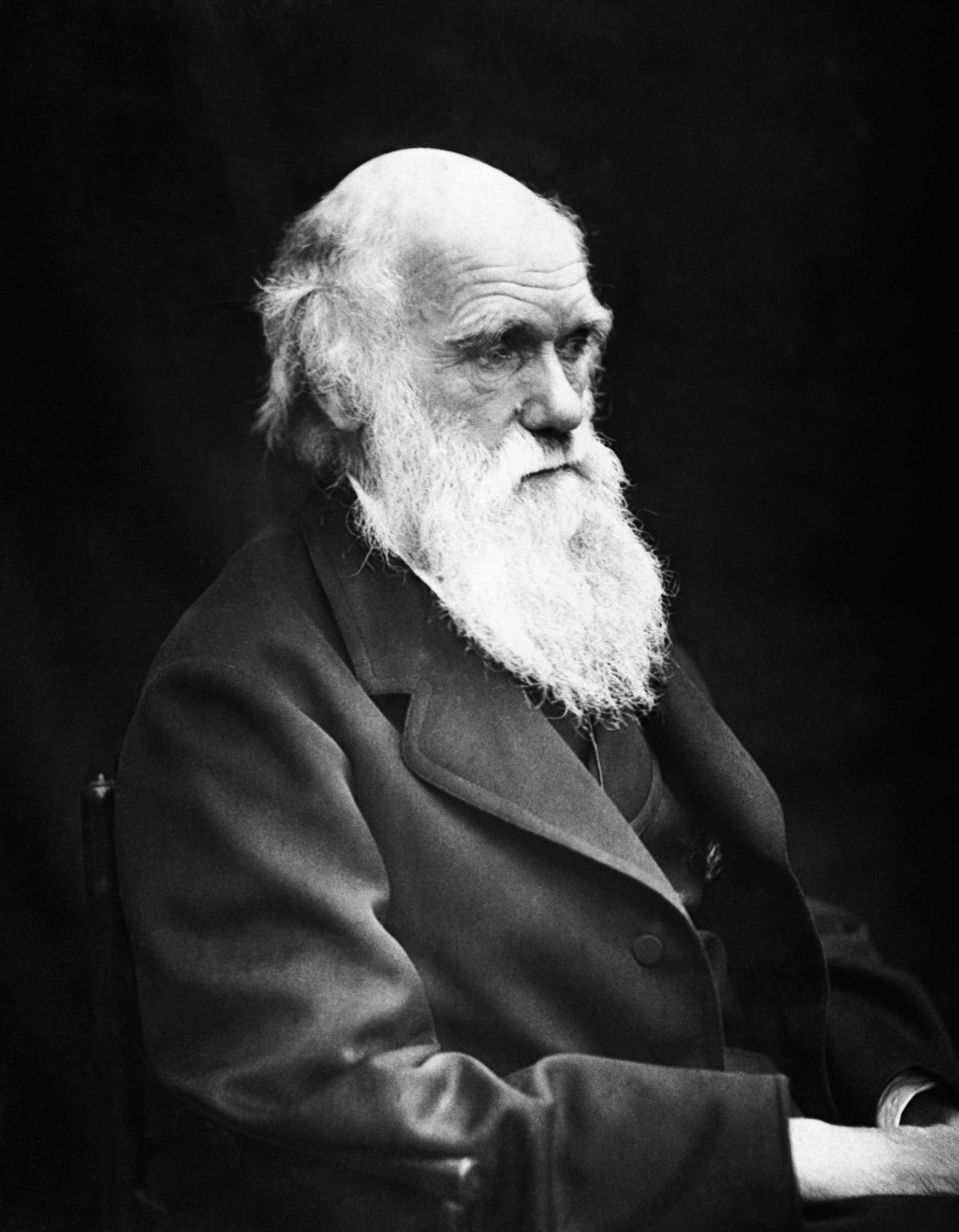
(Image from https://it.wikipedia.org/wiki/Charles_Darwin)
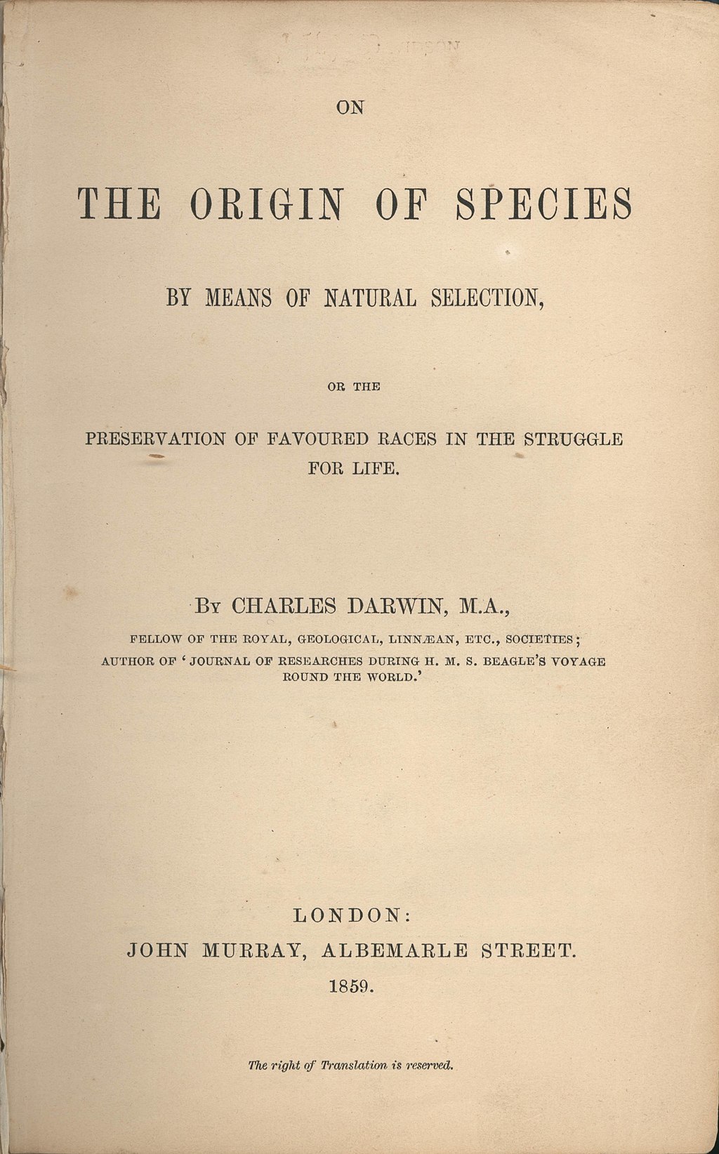
(Image from https://en.wikipedia.org/wiki/On_the_Origin_of_Species)
1.2.2.2. Supporting Decision-Making#
In many cases, data analysis can be used to support decision making. Suppose that we work for a company producing three products A, B and C. The products are sold in three different geographic locations X, Y, Z. Due to the crisis, the company has to reduce the production and wants to cut down one of the three products, but of course they would want to choose the product to stop producing in a way to loose as little earnings as possible. A possible option could also be to keep the three products but reduce the amount of units produced during the year. Fortunately, the company has historical data of productions and sells in the last 5 years. In contexts like these, we could use data analysis techniques to understand which is the best decision to take. Some data analysis techniques could also allow us to make some simulations of what could happen if we took one decision or another.
1.2.2.3. Making Predictions on Unseen Data#
Another typical goal of data analysis is the one of creating models able to make predictions on unseen data. Imagine you are working for a bank which wants to develop an algorithm capable of understanding whether a given transaction is a legitimate one or a fraud attempt. The bank already has a team which reviews the some of the transactions to check if they are legitimate. This is done by checking things such as if the beneficiary of a given transaction is an unusual one, if the beneficiary is notably not to be trusted, and if too many transactions are performed in a given amount of time. If we had past observations of transactions and a variable telling us which of those turned out to be a fraud attempt, we may use data analysis to create a predictive algorithm capable of predicting whether a transaction is a fraud attempt by looking at the values of other available variables such as the amount of money, the nationality of the beneficiary, and the number of transactions made in the last 24 hours.
1.2.3. Main Types of Data Analysis#
While we have discussed of broad goals of data analysis above, we can divide data analysis processes into five main types (different categorization may be possible, but we will stick to this one in this course). Each category describes a mindset and a set of tools that can be used to perform data analysis processes towards the accomplishment of one or more of the goals above. It should be clear that, during a data analysis process, one may mix the different kinds of data analysis or perform them in a sequential fashion. As we will see, the different approaches also rely on similar statistical techniques and one approach does not exclude the others.
The main types of data analysis are:
Descriptive analysis;
Exploratory analysis;
Inferential analysis;
Causal analysis;
Predictive analysis;
Time series analysis.
Let’s briefly see what these types of data analysis are, but we will analyze in greater detail each of these approaches during the course.
1.2.3.1. Descriptive Analysis#
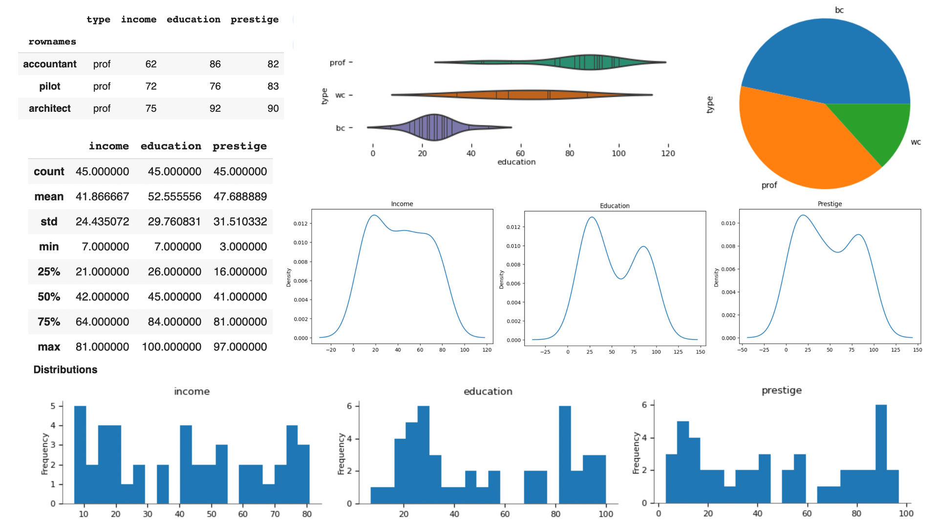
The goal of descriptive analysis is to provide a series of numbers or visualization of the data that describe their main characteristics. The goal is provide a compact summary of the main characteristics of the data. Examples of this kind of analysis including computing the proportion of males and females in the dataset of students and marks, the average marks that each course gets, etc. At this stage, we are not interpreting the results, but only providing some quantitative or qualitative measures of some property. One may think that the best description of some data is the data itself, and that would not be too far from the truth! However, in some cases, it is useful to provide summary statistics which are not evident from the data to start getting a sense of it.
The image in the following shows some examples of descriptive statistics and visualizations extracted from a dataset. We will get more into the details of such techniques later in the course.
1.2.3.2. Exploratory Analysis#
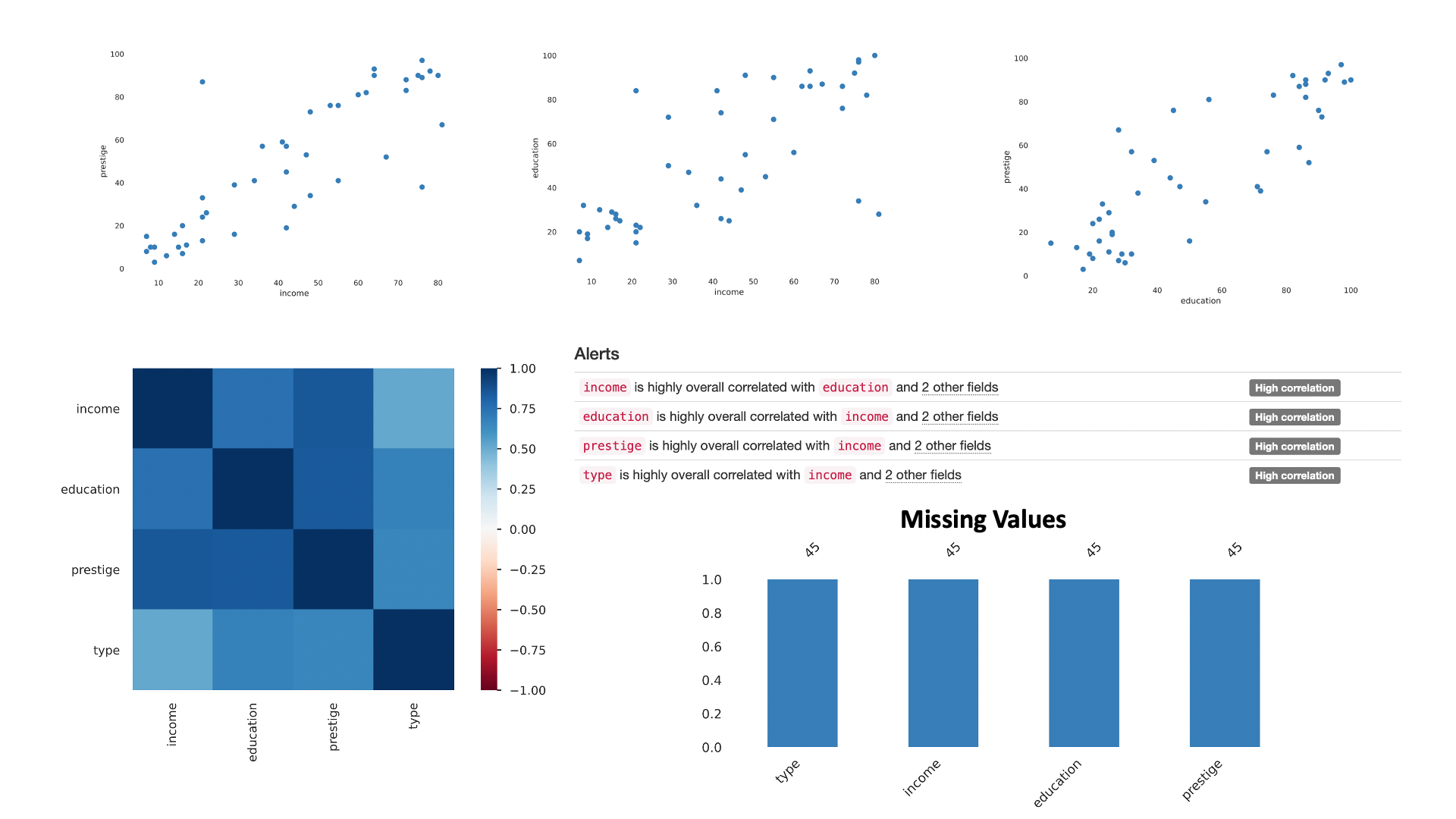
Exploratory analysis aims to examine the structure of the data, the distributions of variables (e.g., how do marks distributes for Physics? What is the average mark?) and the relationships between two or more variables (e.g., do students who have low marks in Physics also get low marks in Mathematics?). As we will see, visualizations are a useful tool for exploratory data analysis, mainly because they are often easy to intuitively absorb. Exploratory data analysis can have different goals, including finding problems in the data (e.g., out of range values, incorrect values, etc.), determining whether the data is good for the analysis we have in mind, making initial hypothesis on which data analysis questions we’ll be able to answer with the data. Importantly, at this stage we are already aiming to find patterns in the data, even if we are keeping our analysis at an informal level.
The image in the following shows some examples of visualizations for exploratory data analysis.
1.2.3.3. Inferential Analysis#
The goal of inferential analysis is to show formally whether some feature of pattern that we are observing in our dataset is actually likely to be true outside of the dataset at hand. Let’s say we are exploring a set of data of people with their daily average consumption of sugars and whether they have diabetes. We may find by looking at the data that people who consume a lot of sugar are more likely to get diabetes. We may be tempted to claim that what we have found a general conclusion, which may apply to the general population (beyond the set of data we are considering). Statistical inference, give us the mathematical tools to check if this generalization is actually possible. For instance, if we had only \(100\) rows in our dataset, we may be suspicious that our conclusion does not apply to the general case and we may want to invest more time in collecting additional data. But, how much data is enough? An inferential analysis will allow us to also check that.
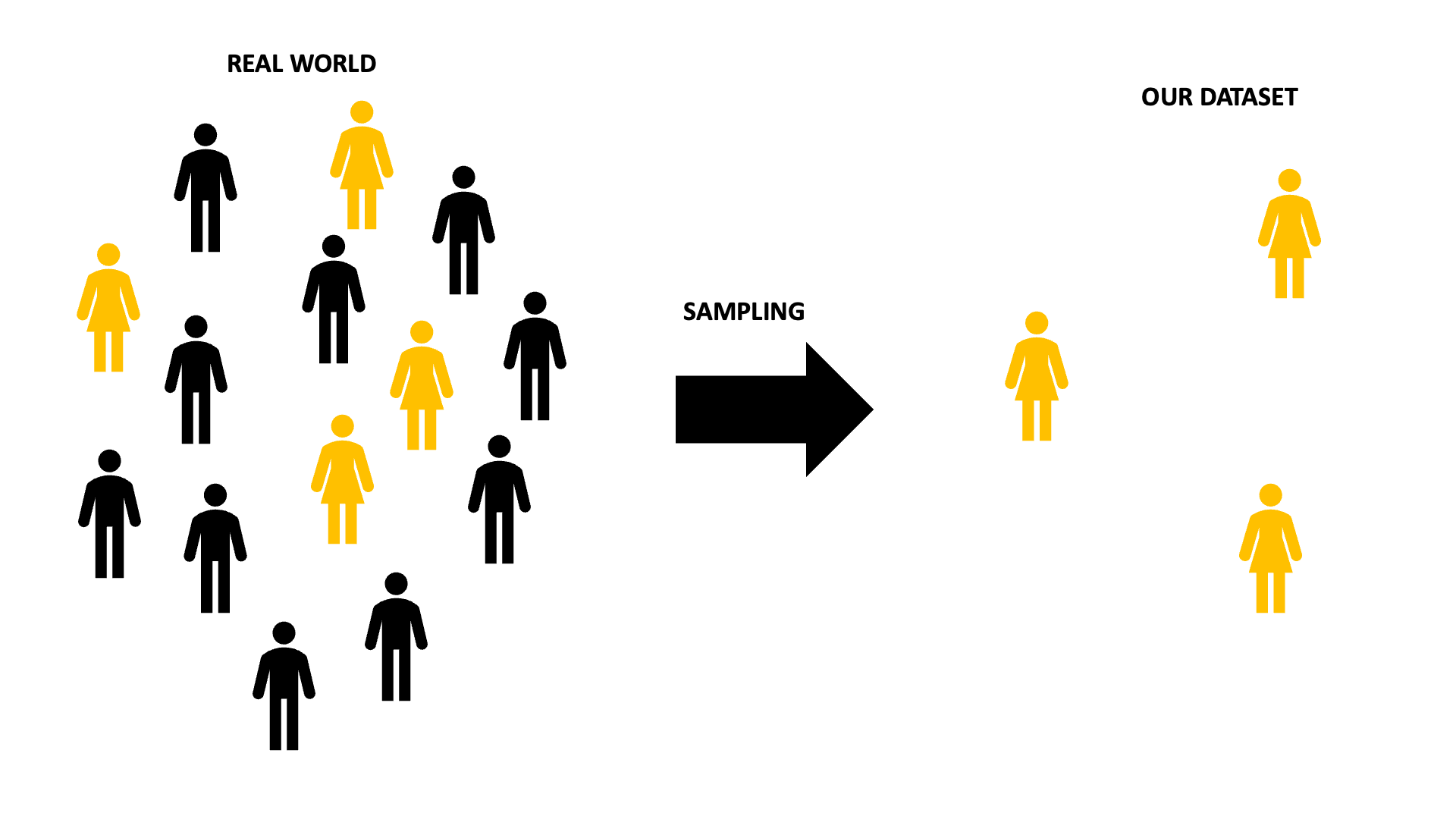
The figure below shows how the sampling process can lead to a dataset which is not an accurate picture of the real world. Inferential analysis aims to check if any conclusion we are drawing based on our data is likely to be true outside of the dataset.
1.2.3.4. Causal Analysis#
While an inferential analysis may allow us to conclude that older people are more likely to develop diabetes and it may even concludes that this apply to the general population, we still don’t know if it safe to say that sugar actually causes people to develop diabetes. This would be an important conclusion. If we knew for certain that consuming more than a given amount of sugar per day would lead to diabetes, than we could enforce some kind of policy to allow people to get the disease. Examples of policies may including classifying foods by their amounts of sugar, so that people can easily know which foods are more dangerous. But what if there is no causal relationship between the consumption of sugar and getting diabetes? For instance, it could just be that people who get diabetes also have a very sedentary life and people with a very sedentary life tend to eat more sugars (e.g., just to get distracted). If this were true, than, it could just be that being sedentary causes diabetes and since being sedentary is associated with eating more sugar, then we were observing an apparent causal effect between eating sugar and getting diabetes. If the second hypothesis is true, then there is no need to classify foods etc. (actually, this may even be undesirable and damage the market). Causal analysis give us tools to determine if a causal effect between two events exist, beyond what we simply observe in the data.
The figure below illustrates how observing some data may suggest that believing in evolution impacts the richness of a country. However, we can probably imagine that other factors may contribute to the observed correlation (more on this later), which might not be due to a cause-effect mechanism.
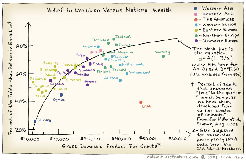
(Image source: https://www.flickr.com/photos/jurvetson/5955305490)
1.2.3.5. Predictive Analysis#
The goal of predictive analysis is to form a model able to predict some unobserved features in data which may be available in the future. Let’s say that we also captured other variables in our example diabetes dataset, such as sex, age, job, etc. We suspect that part of the member of the community may have diabetes and we would like to screen them. However, we cannot just screen all of them (that would be too much and we don’t have enough resources). We may hence think to prioritize the subjects who are more likely to develop diabetes. But who are those? A causal analysis may have revealed that easting too much sugar may be a cause of developing diabetes, but we also have more variables we are capturing. While it is very unlikely that sex of age are causing diabetes, we may observe that, for some reason, older females tend to develop diabetes more often. Predictive analysis allow us to create models that allow to predict a given variable from a set of other variables. For instance, I could create a model which predicts the probability of developing diabetes from sex, age and job. Let’s say I have a list of potential people to screen with the three variables above captured, but I was not able to collect the amount of sugar they consume (note that this is much harder to obtain), then I could use my model on each row to predict what is the probability of each person to develop diabetes. I could then start by screening people with high predicted probabilities of developing the disease. Note that predictive analysis does not care about causal effects and does not rely on inferential analysis to check if our assumptions are valid beyond the dataset, however, it still requires to work for data which have never been seen before. In practice, while we may create our model based on our dataset, we are really interested in using it on data which is not already captured in our dataset (for those in the dataset, we already know who has diabetes).
In the example below, predictive analysis can allow to predict “group” from the other variables for those subjects for which the group is unknown (???).
relwt |
glufast |
glutest |
instest |
sspg |
group |
|---|---|---|---|---|---|
1.06 |
96 |
465 |
237 |
111 |
Chemical |
1.09 |
110 |
426 |
117 |
118 |
Normal |
0.93 |
93 |
472 |
285 |
194 |
??? |
0.92 |
300 |
1468 |
28 |
455 |
Overt |
0.88 |
99 |
376 |
134 |
80 |
Normal |
1.1 |
107 |
403 |
267 |
254 |
Normal |
0.98 |
130 |
670 |
44 |
167 |
??? |
1.13 |
92 |
476 |
433 |
226 |
Chemical |
1.0 |
102 |
378 |
165 |
117 |
Normal |
0.96 |
78 |
290 |
136 |
142 |
??? |
1.2.3.6. Time Series Analysis#
Time series analysis aims to analyze data points recorded over of sequence of intervals to uncover patterns, trends, seasonality, and other characteristics of the data and to make forecasts based on historical data. For example, imagine a retail store which wants to make a forecast to predict sales for the next year. By analyzing the last five years of their sales, the store can use time series analysis to visualize the data, analyze trends (e.g., if sales are globally increasing), analyze seasonality (are there more sales over christmas?), and predict future sales. The predicted sales can be useful to better organize supplies and staff.
The image below shows an example of time series forecasting.
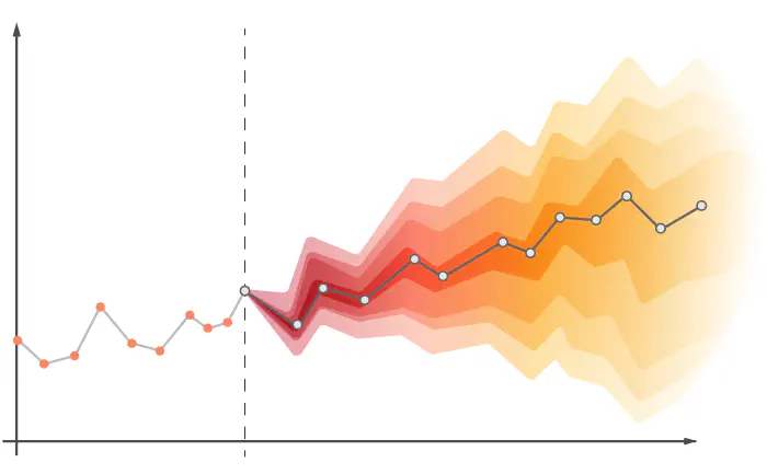
(Image from https://www.lokad.com/probabilistic-forecasting)
1.3. Data Analysis Workflow#
The typical workflow of data analysis is composed of the following stages:
Define your data analysis question
Collect the data needed to answer the data analysis question
Clean and format the data
Explore and describe the data
Choose suitable models for the analysis
Fit, fine-tune, evaluate, and compare the models for the considered data analysis
Review the data analysis when new data is available
Let’s see more in detail what the different steps are about.
1.3.1. Define your data analysis question#
We can see data analysis as the process of answering a question. For instance, in the example above on the theory of evolution, Darwin tried to answer the question “do species appear as an adaptation to features of the environment?”. Similarly, if we perform a causal analysis, we are trying to answer a question such as “does consuming too much sugar causes diabetes?” and if we perform a predictive analysis, we want to answer questions such as “What is the probability that this subject will develop diabetes?”. If we see data analysis as the process of answering questions, the very first step in the data analysis process is to state the question in a way that it is accurate and can be answered with the data. We may revisit this step to refine the question based on what we discovered from the analysis performed so far.
1.3.2. Collect the data needed to answer the data analysis question#
In this stage, we will collect the data we need to answer the data analysis question. If we want to assess whether consuming too much sugar can cause diabetes, we could look for surveys already made on the topic, or we could set a study in which we go around and ask people what are their eating habits.
1.3.3. Clean and format the data#
The collected data does not always come in a “clean” form. In particular, we could have missing data, due to errors in the data collection or people uwilling to answer all questions. For instance, we may ask for age, but some subjects may refuse to tell us which is their age. In other cases, we may have outliers, i.e., “strange” numbers probably due to errors in data collection. For instance, if we find an age of 156 years, that may just be a typo and the intended age was just 56 years. In this stage, we will use a set of techniques to fix these problems in order to filter or clean the data.
1.3.4. Explore and describe the data#
This step consists in exploring the data to make sure that it can be used to answer the question. For instance, we may want to check if the data has been collected properly to answer our question, if it is of sufficient quantity and quality. We will also start to see informally if the question we choose can be plausibly answered with this data.
1.3.5. Choose suitable models for the analysis#
In this stage, we will select a set of models which seem to be suitable for answering our question. For instance, if we want to assess if we can predict whether a give subject will develop diabetes, we could choose classification models. The choice of the specific classification model will also be based on our understanding of the data (e.g., is the problem multi-dimensional? do we have enough data? etc.).
1.3.6. Fit, fine-tune, evaluate, and compare the models for the considered data analysis#
In this stage, we fit the chosen models to the data. After fitting them, we will need to evaluate how well they model the data. In many cases, we will fit more than one model and compare them to decide which of them is the most appropriate.
1.3.7. Interpret the results#
Once models have been built, we need to interpret our results in order to answer our question. For instance, we may observe a causal relationship between consuming sugars and developing diabetes, but we still need to interpret this result to get an understanding of why and how this happens.
1.3.8. Communicate your results#
This stage is concerned with communicating the results of our analysis in an most accurate and understandable way. The way in which we communicate may depend on the specific audience we are talking to. We will use an informal language if the audience is general and non-technical, or a more technical one if we are writing the results of our analysis in a research paper.
1.3.9. Review the data analysis when new data is available#
At some point, new data may be available. In this stage, we should revise our analysis and update our question, answer, or choice of models.
1.3.10. Non-Linear Workflow#
It should be noted that the process is not exactly linear. A good data analysis will iterate over the different steps and possibly jump back to any of those steps to revise it. For instance, after fitting the models on the data in step 5, one may note that some other models could give better results, and jump back to step 4 to refine the choice of the models, to then return to step 5.
The figure below shows the described workflow. Solid arrows illustrate the main flow, while dashed arrows show possible alternative paths after performing data exploration (step 4). Similar dashed arrows pointing to any past node may apply to the other nodes as well. In the example below, after exploratory data analysis (step 4), we may note that the data is not clean (maybe we find some outliers) or not adequately formatted, so we jump back to step 3. Similarly, we may find that we need more data, and jump back to step 2, or we may want to revisit and refine our data analysis question (step 1).
1.3.11. Example#
A data analyst working for an e-commerce company is tasked with analyzing customer reviews to improve product quality and customer satisfaction. The analyst starts by defining the question that the data analysis needs to answer (step 1 - define your data analysis question): “What are the common themes and issues in customer reviews, and how can we address them to improve product quality and satisfaction?” To answer this question, the analyst collects a diverse dataset of customer reviews from various sources (step 2 - collect the data needed), including the company’s website, social media, and third-party review platforms. This dataset includes text reviews, ratings, and timestamps.
Once the data is collected, the analyst proceeds with data cleaning and formatting (step 3 - clean and format the data) since the initial dataset is messy with spelling errors, duplicate reviews, and inconsistent formatting. This involves data preprocessing, such as removing punctuation and converting text to lowercase. After cleaning the data, the analyst explores and describes it (step 4 - explore and describe the data) using techniques like word clouds, frequency distributions, and sentiment analysis to uncover common words, sentiments, and trends within the reviews.
To extract more meaningful insights from the text data, the analyst decides to apply natural language processing (NLP) techniques (step 5 - choose suitable models for analysis). Specifically, Latent Dirichlet Allocation (LDA) for topic modeling is chosen to identify recurring themes within the reviews. However, upon implementing LDA and reviewing the results, the analyst realizes that some topics are unclear and overlapping (step 6 - fit, fine-tune, evaluate, and compare the models).
Acknowledging the need to revisit the analysis, the analyst decides to backtrack to the data exploration step (step 4 - explore and describe the data) to gain a deeper understanding of the customer feedback. During this reassessment, it becomes evident that customers frequently mention product quality issues when discussing customer service experiences, leading to topic overlap. Armed with this insight, the analyst decides to categorize reviews into “product-related” and “service-related” (step 5 - choose suitable models for analysis) before applying topic modeling.
With the revised approach, the analyst proceeds to categorize reviews and then applies LDA separately to the two categories (step 6 - Fit, fine-tune, evaluate, and compare the models for the considered data analysis). This results in more interpretable topics, such as “defective products,” “timely shipping,” and “responsive customer support.” The analyst then analyzes these topics to generate actionable insights for product improvement and customer service enhancements.
To ensure continuous improvement, the analyst commits to ongoing review and monitoring (step 7 - Review the data analysis when new data is available) of customer reviews, periodically updating the analysis to identify new emerging issues or trends. This iterative approach to data analysis allows for refining strategies and addressing evolving customer concerns over time.
1.4. Examples of Data Analysis: the Good, the Bad, and the Ugly#
Before concluding this introduction, we will analyze and discuss some notable examples of data analyses. Since we don’t have any theoretical or technical tool to understand these analysis in depth, we will just focus on the stories behind these analyses and their main outcomes.
It is important to emphasize that analyzing data is a complex process, hence it is prone to error. Moreover, when collecting data about people, such as their preferences and tastes, we should be careful of what kind of conclusion we draw from the analysis and what we do with the data. Keeping these pitfalls in mind, we will discuss three examples of data analysis, a good example in which data analysis can be used to make decisions and save lives, a bad example in which data analysis has been intentionally used to lie and deceive, and an ugly example in which data analysis has probably been performed in a technical correct, but unethical way.
These example are meant as a way to illustrate the power of data analysis and warn about the pitfalls and ethical implications.
1.4.1. The Good: Stopping the Spread of Cholera#
In the nineteenth century, cholera pandemics were common, but little was understood about them. A common belief was that cholera pandemics was caused by “miasma”, particles in the air carrying the disease (see Fig. 1.1). This was justified by the observation that pandemics tended to be localized, meaning that people getting the disease were living in the same house or neighborhood.
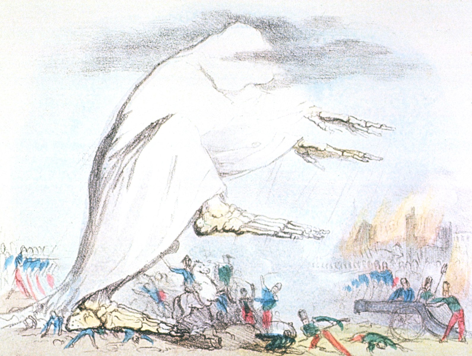
Fig. 1.1 A 19th century color lithograph by Robert Seymour depicting cholera as a skeletal creature emanating a deadly black cloud, based on the popular belief of miasma. Image from https://en.wikipedia.org/wiki/Miasma_theory.#
In 1854, John Snow (See jonsnow), an English doctor, hypothesized that, instead, pandemics were due to the contamination of water with the contents of the sewer’s system.
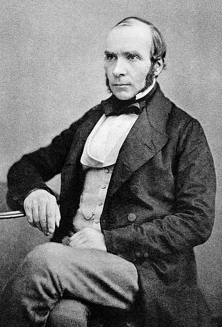
Fig. 1.2 John Snow (1813 – 1858) was an English physician and a key figure in the development of anaesthesia and medical hygiene. Image from https://en.wikipedia.org/wiki/John_Snow.#
When a severe outbreak of cholera started in Broad Street in London, John Snow started to analyze the deaths due to cholera and put them on a dot distribution map, which was later known as the “Ghost Map” (see ghostmap), since it took track of how many people died in a given place of the map. To collect, the data, John Snow interviewed local residents with the help of Reverend Henry Whitehead.
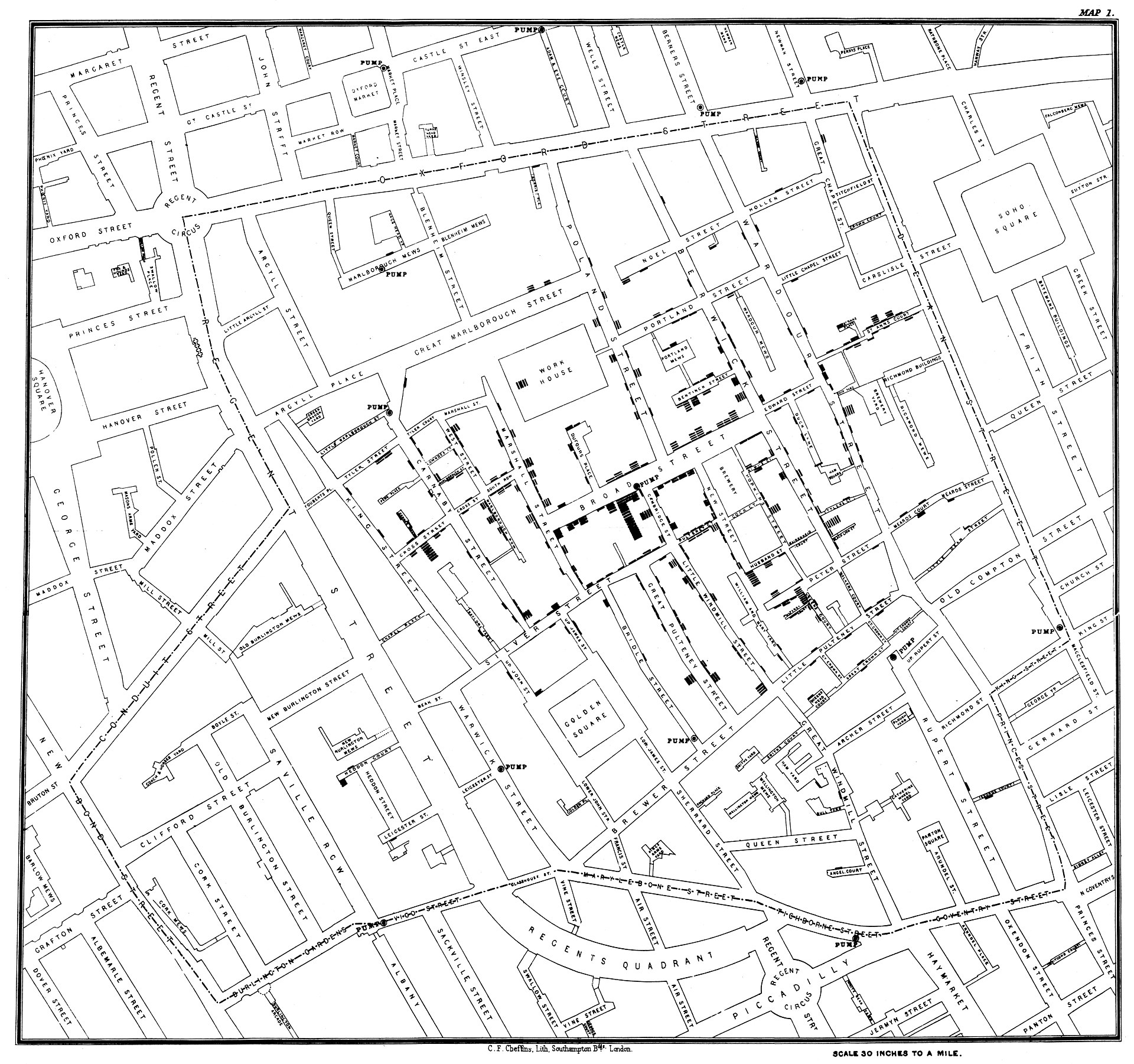
Fig. 1.3 The ghost map made by Jon Snow to study the cholera outbreak. Image from https://en.wikipedia.org/wiki/1854_Broad_Street_cholera_outbreak#
In the map, bars represented the deaths, while circles represented the positions of public water pumps. At the time, people did not have water in their homes, hence they had to reach water pumps and get water from there. John Snow computed the distance of each of the houses to each water pump in the area and noted that for places with more deaths, the closest pump was located in Broad Street.
Based on this evidence, John Snow managed to convince the authorities to remove the handle of the pump, hence forcing people to take water from somewhere else. John Snow noted a drastic reduction in the number of deaths in the subsequent days. Since the water coming to the surrounding pumps was from the same source, Snow concluded that the pipes connected to pump in Broad Street must have been contaminated with sewage.
After the cholera epidemic stopped, government officials replaced the pump handle, refusing John Snow’s theory. It will take time for his theories to be accepted.
In 1992, a replica of the pump with the handle removed was installed at the site of the 1854 pump (figure Fig. 1.4).

Fig. 1.4 The replica of the pump with the handle removed installed in 1992. Image from https://en.wikipedia.org/wiki/1854_Broad_Street_cholera_outbreak#
1.4.2. The Bad: Proving Nonexistent Links Between MMR Vaccines and Autism#
In 1998, Andrew Wakefield and twelve coauthors published a paper entitled “Ileal-lymphoid-nodular hyperplasia, non-specific colitis, and pervasive developmental disorder in children” in The Lancet (one of the most important medical Journals). The paper claimed the existence of a causative link between the MMR vaccine and colitis and between colitis and autism.
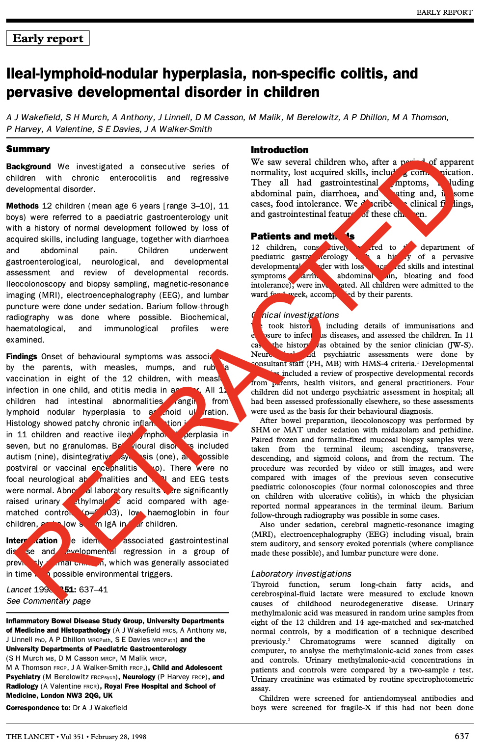
Fig. 1.5 The paper published in the Lancet, and later retracted. From https://www.thelancet.com/journals/lancet/article/PIIS0140673697110960/fulltext.#
Several studies (at least 20) tried to replicate Wakefield’s study and where not able to show any link between vaccine and autism, hence assessing that there is no associated between the two.
Some facts about the paper:
The study was based on 12 children, which had been carefully selected to allow to verify the claim. Many of their parents already believed that the MMR vaccination had caused their children’s autism.
Wakefield had not disclosed a serious financial conflict: he had been paid by lawyers involved in lawsuits against immunization manufacturers and was applying for a new vaccine patent.
In 2004, 10 of the 13 authors retracted their support for the MMR-autism association.
Britain’s General Medical Council investigation found Wakefield guilty of dishonesty and irresponsibility.
In 2010, the Lancet fully retracted the Wakefield study (see The paper published in the Lancet, and later retracted. From https://www.thelancet.com/journals/lancet/article/PIIS0140673697110960/fulltext.).
Despite the fraudulent nature of this data analysis has now been uncovered, the paper had a profound impact on the rate of immunizations which decreased dramatically, with increased risks for children (see MMR vaccination coverage in relationship with the publication of Wakefield’s paper. © Tangled Bank Studios; data from the National Health Service of the United Kingdom. Image from https://www.pbs.org/wgbh/nova/article/autism-vaccine-myth/).
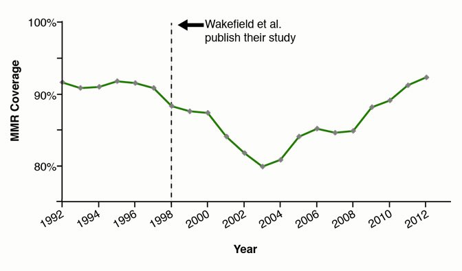
Fig. 1.6 MMR vaccination coverage in relationship with the publication of Wakefield’s paper. © Tangled Bank Studios; data from the National Health Service of the United Kingdom. Image from https://www.pbs.org/wgbh/nova/article/autism-vaccine-myth/#
This is an example of how a fraudulent data analysis can be crafted in a convincing way (the paper was accepted by The Lancet!) and what kind of damage it can do to society.
More information about this story here:
1.4.3. The Ugly: Manipulating Voters with Stolen Data - The Facebook-Cambridge Analytica Scandal#
In 2013, a company called Cambridge Analytica (Fig. 1.7) was founded with the intention of utilizing data analysis and strategic communication to influence political campaigns. Their claimed expertise lay in psychographic profiling, a method that categorizes individuals based on their psychological traits and behaviors.

Fig. 1.7 Image from https://en.wikipedia.org/wiki/Cambridge_Analytica#
In 2014, Aleksandr Kogan, a researcher at Cambridge Analytica, developed an app named “This Is Your Digital Life.” On the surface, it appeared to be a harmless personality quiz. However, without the consent of the users, the app collected not only their personal data but also the information of their Facebook friends.
Through the “This Is Your Digital Life” app, Cambridge Analytica gained access to an astonishing amount of personal data. They obtained profiles from around 87 million Facebook users, obtaining a vast quantity of information including public profiles, likes, preferences, and more.
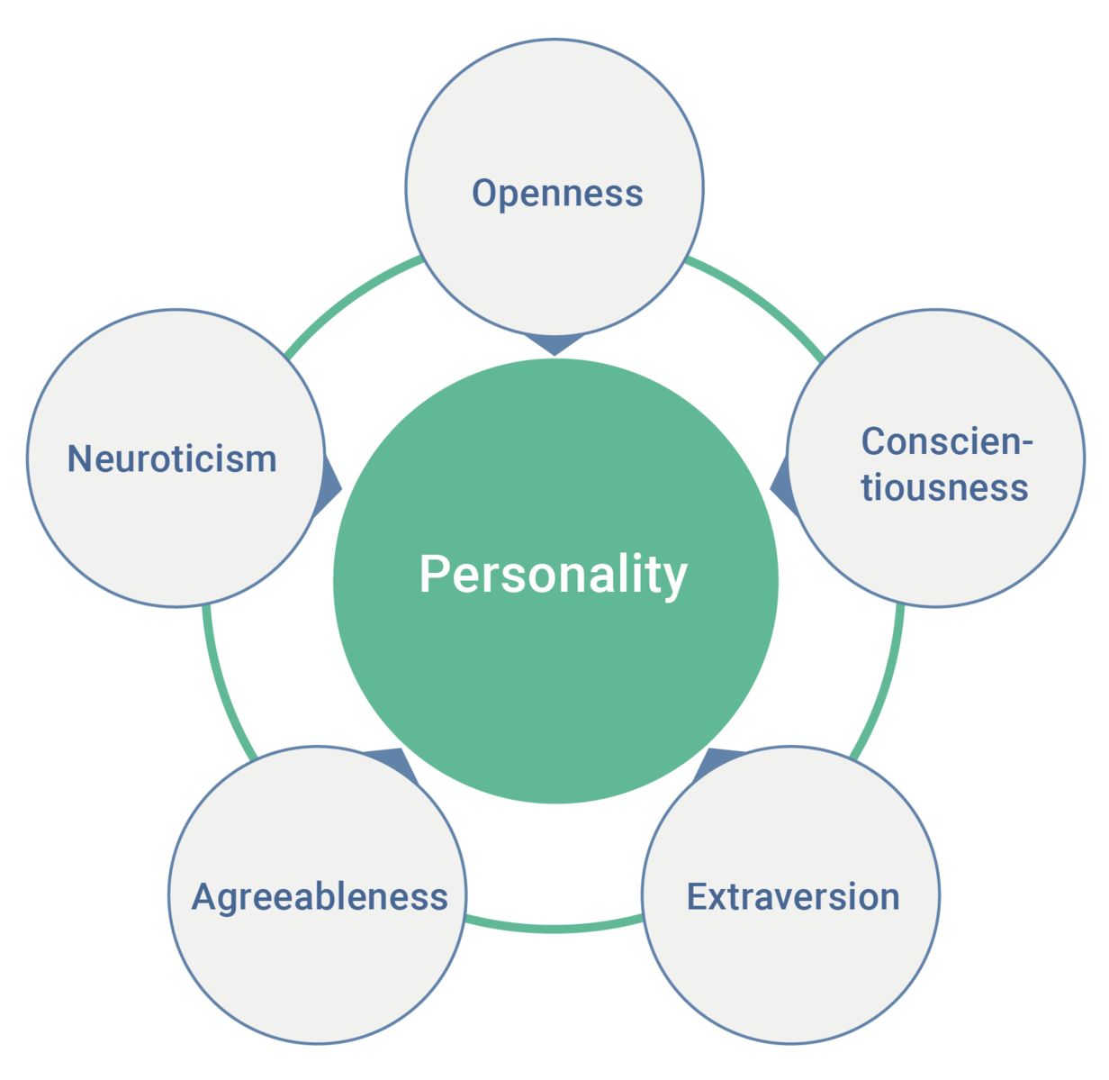
Fig. 1.8 Image from https://commons.wikimedia.org/wiki/File:Wiki-grafik_peats-de_big_five_ENG.png#
Based on this data, Cambridge Analytica employed data analysis techniques to construct detailed psychological profiles of individuals using the Big Five personality traits model (see Fig. 1.8). They claimed to possess thousands of data points on each person, enabling them to tailor political messages and advertisements to specific personality types.
As Alexander Nix, the chief executive of Cambridge Analytica claimed:
Today in the United States we have somewhere close to four or five thousand data points on every individual … So we model the personality of every adult across the United States, some 230 million people.
(Source https://en.wikipedia.org/wiki/Cambridge_Analytica)
The unethical aspect of Cambridge Analytica’s actions lay in their misuse of personal data obtained without proper consent. Furthermore, their involvement in political campaigns raised concerns about potential manipulation of democratic processes through targeted misinformation and propaganda.
The scandal erupted into the public eye in 2018, when investigations exposed Cambridge Analytica’s practices. The revelation sparked a massive outcry over privacy violations, ethical standards, and the regulation of data analytics. Facebook, being the platform from which the data was harvested, faced intense scrutiny for their failure to safeguard user data and prevent unauthorized access. The scandal triggered investigations by regulatory bodies and lawmakers, leading to increased calls for stricter data protection regulations.
The story of the Cambridge Analytica scandal is a good example of the risks associated with unethical data practices.
1.5. What’s Data Analysis Used For Today#
Data analysis is used today in a number of contexts, which makes the job of the data analysts highly sought after by companies. Some examples are in the following.
1.5.1. Healthcare#
Data analysis plays a crucial role in healthcare, enabling insights that can improve patient outcomes and optimize operations. For example, predictive analysis can be used to identify patients at high risk of developing specific diseases, such as diabetes or heart disease, allowing healthcare providers to intervene early with preventive measures. Additionally, analyzing electronic health records and medical imaging data can aid in diagnosing diseases, developing personalized treatment plans, and identifying patterns that may improve overall healthcare delivery.
1.5.2. Retail and E-commerce#
Data analysis has revolutionized the retail and e-commerce industry. Companies like Amazon utilize data from customer browsing behavior, purchase history, and demographic information to create personalized product recommendations. By analyzing customer data, retailers can optimize pricing strategies, manage inventory more effectively, and forecast demand. Furthermore, sentiment analysis of customer reviews and social media data can provide valuable insights into consumer preferences and help improve product development and marketing campaigns.
1.5.3. Financial Services#
Data analysis is instrumental in the financial services industry for fraud detection, risk assessment, and investment decision-making. Banks and credit card companies employ data analytics to identify fraudulent transactions by analyzing patterns, anomalies, and behavioral data. Risk models that analyze historical data and market trends are used to assess creditworthiness and make lending decisions. Moreover, algorithmic trading leverages complex data analysis techniques to identify market trends and make high-speed trading decisions.
1.5.4. Transportation and Logistics#
Data analysis is used extensively in transportation and logistics to optimize routes, reduce costs, and improve overall efficiency. For instance, ride-sharing platforms like Uber and Lyft leverage data analysis to match drivers with riders efficiently and minimize wait times. Logistics companies employ route optimization algorithms to minimize fuel consumption and reduce delivery times. Real-time data analysis of traffic patterns and weather conditions helps improve route planning and avoid delays.
1.5.6. Process Optimization#
Chip manufacturers collect vast amounts of data at various stages of the manufacturing process. This data includes measurements from sensors, equipment logs, and performance metrics. By analyzing this data, engineers can identify patterns, correlations, and anomalies that can lead to process optimization. For instance, data analysis can be used to identify parameters that significantly impact chip yield and quality. By analyzing historical data, engineers can uncover trends and relationships between process variables and chip performance. This information can then be used to optimize process settings, reduce defects, and improve overall chip quality.
1.5.7. Fault Detection and Predictive Maintenance#
Data analysis techniques such as machine learning can be applied to detect faults and predict equipment failures in chip manufacturing. By analyzing sensor data from production equipment, anomalies or deviations from normal operating conditions can be identified in real-time. Through predictive maintenance, engineers can leverage data analysis to detect early signs of equipment degradation or impending failures. By analyzing historical maintenance records and equipment sensor data, patterns can be identified to predict when maintenance is required. This proactive approach minimizes unplanned downtime, maximizes equipment utilization, and reduces production losses.
1.5.8. Solar Energy Optimization#
Data analysis is instrumental in optimizing the efficiency and output of solar energy systems. Solar farms and rooftop solar installations can generate large amounts of data, including solar irradiance levels, weather patterns, system performance metrics, and energy production data. By analyzing this data, solar energy operators can identify patterns and trends in solar irradiance, weather conditions, and energy production. This information can be used to optimize the positioning of solar panels, adjust tilt angles, and improve maintenance schedules. Data analysis can also help predict energy generation and optimize energy storage systems, ensuring maximum utilization of solar resources.
1.5.9. Energy Grid Optimization#
Data analysis can help optimize the performance and stability of energy grids with a high penetration of renewable energy sources. By analyzing real-time data on energy generation, consumption, and grid conditions, operators can identify potential issues, manage grid stability, and improve energy flow. Data analysis techniques, such as machine learning algorithms, can be applied to detect anomalies, predict grid congestion, and optimize grid operation. This enables grid operators to proactively address challenges, integrate renewable energy sources efficiently, and enhance the overall reliability and resilience of the energy grid.
1.6. Where do We Go From Here?#
I hope this introduction has set the ground and created some (hopefully positive!) expectation on what we are going to learn in the course. We should now briefly touch on how we are going to do it within this course.
1.6.1. Philosophy of the Course#
Data analysis is a complex process involving different theoretical concepts with roots in well established theoretical fields such as that of statistics. While it is fundamental to understand the theoretical premises and assumptions, we will opt for a formal, but practical introduction of these concepts. This means that we will introduce and describe models, but we will not delve too deeply into the mechanics of optimization of the models or demonstration of theoretical guarantees. At the same time, while we will rely on libraries to use the models and techniques introduced in the course, we will aim to forming a deep and formal understanding of how a given algorithm works. This is fundamental to understand when a given tool should be used and when it should not be used.
1.6.2. Practical Data Analysis with Python#
Since data analysis is a practical process, we will also rely on laboratories to introduce, understand and play with models, algorithms and concepts whenever appropriate. We will use the Python programming language and different Python libraries explicitly designed to perform data analyses. Another popular choice for data analysis is the R software. Both options (Python and R) are valid but the two packages follow different approaches:
R has been introduced as a statistical language for non-technical people. Hence the focus was on the ease of use and attention on the process rather than on the programming side of the language itself. While R is probably the best supported language for statistical and data analysis (with a lot of great libraries explicitly designed for that), the language may appear not very flexible to people with a programming background.
Python has been introduced as a general purpose programming language and became popular as a software for scientific computation and data analysis. Since it is a general purpose programming language, is is very flexible, even supporting multiple programming paradigms such as procedural, object oriented, and functional. The downside is that the language has not been explicitly designed for data analysis, so those functionalities are offered by external libraries which address specific data analysis aspects and are not always super-coherent with respect to their APIs and general approach.
That said, both solutions allow to achieve the same results. In this course we opt for Python as it will probably feel more natural to computer science course. Moreover, while Machine Learning is outside the scope of this course, Python is the main language for Machine Learning, so learning it will prove very useful for students who wish to take Machine Learning courses in the future.
1.6.3. A Map of the Course#
I hope this introductory lecture has sparked some interest on the fascinating topic of data analysis. While data analysis is a practical field, a data analyst is still required to have some solid formal understanding on how and why the algorithms and models used for data analysis work. This will also be useful to develop an intuition of what may go wrong in a data analysis, which, as the examples above have shown, is an important ability to gain.
We plan to address the different topics of the course by following the different kinds of data analysis that can be made. Hence, the course will develop through the following macro-units:
Descriptive and exploratory analysis. We put both analyses types in the same unit as the tools for these two kinds of analysis are sometimes shared, even if their objectives are distinct.
Inferential analysis. We will see what are the main tools to make sure that any conclusion we are drawing on the data will likely apply beyond the data that we are analyzing.
Causal analysis. We will just give an introduction here. The topic is broad and an entire course could be devoted to it. Here we aim to identify the main pitfalls so that we can be aware of which mistakes we can incur in without a proper data analysis. We will also see some simple approaches which may be sufficient in some cases to perform a proper causal analysis.
Predictive analysis. We will discuss the philosophy of the approach, which is rather different from the different kinds of analysis seen above, revisit some of the algorithms discussed in the previous sections according to the predictive paradigm and see some powerful predictive algorithms which can be applied for data analysis. While this is not a machine learning course, this part will provide initial tools and lay the grounds for an in-depth understanding of what machine learning (including deep learning) is.
Time series analysis. We will provide an introduction to the analysis of time series, highlighting the main concepts and techniques.
During our journey, we will both focus on theoretical concepts and apply them in practice in real examples of data analyses. This will be done through frequent short laboratory sessions (in the order of one per lecture) showing how to use the introduced concepts in practice, and lectures dedicated to the applications of the discussed concepts in real data analyses.
1.5.5. Social Media and Digital Marketing#
Data analysis plays a crucial role in social media platforms and digital marketing campaigns. Companies analyze user engagement metrics, demographic data, and social media trends to understand customer behavior and tailor marketing strategies. A/B testing is used to compare the effectiveness of different marketing campaigns. Social media sentiment analysis enables businesses to gauge public opinion, manage brand reputation, and identify emerging trends.