6. Probability for Data Manipulation#
In this lecture, we will look at some basic elements of probability theory which will help us manipulate data in a more accurate and principled way.
6.1. Uncertainty & Importance of Probability Theory#
We have seen that dealing with data means dealing with “some variables assuming some values”.
However, what can we say about what values such variables will assume?
In some cases, it is possible to predict the values of these variables with perfect accuracy, given a set of initial conditions. For instance, think about a system of equations describing the speed of objects according to Newtonian laws.
In other cases, modeling the relationship between variables in a deterministic way is not possible. We often say that this is due to uncertainty.
As reported here, uncertainty in a system can be due to different factors:
Inherent stochasticity in the system being modeled. Some events such as drawing a card from a deck of cards, rolling a die, or the movements of subatomic particles can be seen as truly random events. The outcomes of such events cannot be predicted with perfect accuracy, so they are stochastic (random).
Incomplete observability. Sometimes, even in a deterministic system, we cannot observe anything. For instance, in the Monty Hall problem, the participant to the game is asked to choose between three doors. One of the doors contains a prize, while the others lead to a goat. Even if the event is deterministic, the game contestant cannot observe everything, so from their point of view, the outcome is uncertain.
Incomplete modeling. Sometimes a system has to discard some of the information needed to make a decision. For instance, imagine a robotic system aiming to pick objects from a table with a single RGB camera. The system cannot reconstruct the 3D position of the objects, but the RGB camera an allow to obtain an estimate of the 2D coordinates of each objects with respect to the robot’s point of view. All the information which cannot be observed is uncertain, despite the problem is a deterministic one.
6.1.1. Examples#
Tossing a coin or rolling a die: these kinds of experiments are generally impossible to model in a deterministic way. This can be due to our limited ability to model the event (i.e., rolling a die might be deterministic, but deriving a set of equations to determine the outcome given the initial motion of the hand is intractable).
Determining if a patient has a given pathology: different pathologies might have similar symptoms. Hence, observing some of them does not allow to determine with perfect accuracy if the patient has that pathology. In this case, uncertainty might arise from incomplete observability.
6.1.2. Importance of Probability Theory#
Probability theory provides a consistent framework to work with uncertain events.
It allows to quantify and manipulate uncertainty with a set of axioms, as well as to derive new uncertain statements.
Probability theory is hence an important tool to work with data. We will start to revise the main concepts behind probability theory by talking about random variables.
6.1.3. Random Experiments#
In practice, when the acquisition of data is affected by uncertainty, we will use the term random experiment. We will informally define a random experiment as:
An experiment which can be repeated any number of times, leading to different outcomes.
We will use the following terminology:
sample space \(\Omega = \{\omega_1,\ldots,\omega_k\}\): the set of all possible outcomes of the experiment;
simple event \(\omega_i\): a possible outcome of a random experiment;
event \(A \subseteq \Omega\): a subset of the sample space including certain events. We usually denote \(\overline A = \Omega \setminus A\) as the complementary event to \(A\), i.e., the event that \(A\) does not happen.
Given the definitions above, \(\Omega\) is often called the sure event or certain event, because it contains all possible outcomes. The null set \(\emptyset\) is called the impossible event.
6.1.3.1. Example#
Let us consider the random experiment of rolling a die. Our outcomes will be numbers which we read on the top face of the die when it lands. We will have:
Sample space: \(\Omega=\{1,2,3,4,5,6\}\);
Simple event: an example of a simple event would be \(\omega_1=1\);
Event: the event “we obtain 1” could be denoted by \(A=\{1\}\). The event “we obtain an even number” can be denoted by \(A=\{2,4,6\}\). We would have \(\overline A = \{1,3,5\}\), the event that “we obtain an odd number”.
6.2. Random Variables#
We have so far talked about “statistical variables”. When dealing with uncertain events, we need to use the concept of ‘random variables’. Informally (from wikipedia):
A random variable is a variable whose values depend on outcomes of a random phenomenon.
A random variable is characterized by a set of possible values often called sample space, probability space, or alphabet (this last term comes from information theory, where we often deal with sources emitting symbols from an alphabet, in which case the values of \(X\) will be the symbols).
Formally, if \(\Omega\) is the sample space, we will define a random variable as a function:
Where E is a measurable space and often \(E=\mathbb{R}\). This definition is similar to the one of statistical variable we have given before.
A random variable is generally denoted by a capital letter, such as \(X\).
Random variables can be discrete or continuous. Discrete random variables can assume a finite number (or a countable infinite number) of possible values, whereas a continuous random variable is generally associated with a real number.
Random variables can be scalar (e.g., X=1) or multi-dimensional (e.g., \(X = \binom{1}{3}\), or \(X = \begin{pmatrix} 1 & 2 \\ 3 & 4 \\ \end{pmatrix}\)).
A random variable is always related to some uncertain phenomenon which generates observations. This is often referred also as ‘experiment’. For instance, if a random variable takes the values of tossing a coin, then ‘tossing a coin’ is the underlying experiment.
The following table lists some examples (see also descriptions below).
Discrete |
Continuous |
|
|---|---|---|
Scalar |
Tossing a coin |
Height of a person |
Multidimensional |
Pair of dice |
Coordinates of a car |
6.2.1. Example - discrete scalar#
For example, \(X\) may denote the outcome of tossing a coin;
In this context, ‘tossing a coin’ is the random phenomenon characterizing the random variable;
The space of possible values that \(X\) can assume (the alphabet of \(X\)) can be defined as \(\left\{ head,\ tail \right\}\). In this example, \(X\) is discrete;
If tossing the coin, the outcome is \(head\), then the variable \(X\) assumes the value \(X = head\).
6.2.2. Example - continuous scalar#
\(X\) may denote the height in meters of a student in this class;
If we pick a student of heigh 1.75m, then \(X = 1.75\);
6.2.3. Example - continuous multi-dimensional#
\(X\) may denote the latitude and longitude coordinates of a car in the world;
Once we pick a car, we may have \(X = \binom{37}{15}\).
6.2.4. Example - discrete multi-dimensional#
\(X\) may denote the outcome of rolling two dice.
In this context, rolling two dice is the random phenomenon characterizing the random variable.
The space of possible values that \(X\) can assume is \(\left\{ 1,2,3,4,5,6 \right\}^{2}\) (pair of numbers between 1 and 6).
Once we roll the dice, we could have \(X = \binom{3}{5}\).
6.2.5. Urns and Marble Example#
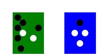
We will now introduce an example that we will use in the rest of this lecture to reason on some basic properties of probabilities. Let’s assume we have two urns urns: one green and one blue.
Each box contains marbles of two colors: black and white.
We consider the experiment of randomly drawing a marble from one of the two urns. This happens in two stages:
We first randomly pick one of the two urns;
Then we randomly pick one of the marbles in the urn;
After observing the type of the marble, we replace it in the same urn.
The outcome of the experiment can be characterized by two random variables:
U represents the color of the urn and can take values g (green) and b (blue).
M represents the color of the marble and can take values b (black) and w (white).
If we pick a white marble from the blue urn, then the outcome of the experiment can be characterized by the values \(M = w\), \(U = b\);
6.3. Working Definition of Data#
We will define “data” as follows:
The values assumed by a random variable
6.3.1. Example#
For instance, if the outcome of tossing a coing is \(head\), then \(X = head\) is data;
It should be clear that the ‘data’ is the pair <random variable, value> and not just the value. Indeed \(head\) alone would not be very useful (we don’t know which phenomenon it is related to), whereas \(X = head\) can be useful, as we know that \(X\) is the random variable describing the outcome of tossing a coin;
In this example, the data \(X = head\) is representing a fact: ‘I tossed a coin and the outcome was \(head\)’. This is also called ‘an event’;
6.4. Probability#
Since random variables are related to stochastic phenomena, we cannot say much about the outcome of a single phenomenon.
However, we expect to be able to characterize the class of experiments related to a random variable, to infer rules on what values the random variable is likely to take.
For instance, in the case of coin tossing, we can observe that, if I toss a coin for a large number of times, the number of heads will be roughly similar to the number of tails.
This kind of observations is useful, as it can give us a prior on what values we are likely to encounter and what are not.
To formally express such rules, we can define the concept of probability on a random variable.
Specifically, it is possible to assign a probability value to a given outcome. This is generally represented with a capital P:
For instance, \(P(U = b)\) represents the probability of picking a blue urn in the previous example;
A probability \(P(U = b)\) is a number comprised between 0 and 1 which quantifies how likely we believe the event to be;
0 means impossible;
1 means certain;
When it is clear from the context which variable we are referring to, the probability can also be expressed simply as:
6.4.1. Probability Axioms#
Kolmogorov in 1933 provided three axioms which define the “main rules” that probability should follow:
Axiom 1 Any event has a probability in the range \([0,1]\):
Axiom 2 The certain event has probability 1:
Axiom 3 If \(A\) and \(B\) are disjoint event (i.e., \(A \cap B = \emptyset\)), then:
From these axioms, the following corollaries follow:
6.4.2. Laplace Probability#
When all outcomes in a random experiment are considered equally probable, this is called a Laplace experiment. In this case, we can calculate the probability of a given event \(A\) as the ratio between the favorable outcomes and the possible outcomes:
For instance, if we are tossing a die:
The probability of obtaining any of the faces will be: \(\frac{1}{6}\);
The probability of obtaining an even number will be: \(\frac{|\{2,4,6\}|}{|\{1,2,3,4,5,6\}|} = \frac{3}{6} = \frac{1}{2}\).
6.4.3. Estimating probabilities from observations#
What about the cases in which we cannot make any assumption on the equal probability of events? In those cases we would like to estimate probabilities from observations. There are two main approaches to do so: frequentist and Bayesian.
6.4.3.1. Frequentist approach#
Probability theory was initially developed to analyze the frequency of events. For instance, it can be used to study events like drawing a certain hand of cards in a poker game. These events are repeatable and can be dealt with using frequencies. In this sense, when we say that an event has probability \(p\) of occurring, it means that if we repeat the experiment infinitely many times, then a proportion \(p\) of the repetitions would result in that outcome.
According to the frequentist approach, we can estimate probabilities by repeating an experiment for a large number of times and then computing:
The number of trials: how many times we performed the experiment;
The number of favorable outcomes: how many times the outcome of the experiment was favorable.
The probability is hence obtained by dividing the number of favorable outcomes by the number of trials.
For instance, let’s suppose we want to estimate the probability of obtaining a ‘head’ by tossing a coin. Let’s suppose we toss the coin 1000 times and obtain 499 heads and 501 tails. We can compute the probability of obtaining head as follows:
Number of trials: 1000;
Number of favorable outcomes: 499.
The probability of obtaining head will be 499/1000=0.49
This is the approach we have seen so far in the course when dealing with relative frequencies.
6.4.3.1.1. Examples#
The probability of obtaining ‘head’ when tossing a coin is 0.5. We know that because, if we toss a coin for a large number of times, about half of the times, we will obtain ‘head’;
The probability of picking a red ball from a box with 40 red balls and 60 blue balls is 0.4. We know this because, if we repeat the experiment for a large number of times, we will observe that proportion.
6.4.3.2. Bayesian Approach#
The Bayesian approach to probability offers a different perspective on probability theory. Unlike the frequentist approach, which focuses on analyzing the frequency of events based on observations, the Bayesian approach allows us to incorporate prior knowledge and update our beliefs as new information becomes available.
In Bayesian probability, we view probability as a measure of uncertainty or belief. When we assign a probability to an event, it reflects our subjective degree of belief in the event’s likelihood. This approach is particularly useful when dealing with unique or one-time events where frequency-based analysis may not be applicable (e.g., “what is the probability that the sun will extinguish in 5 billion years?”).
We will discuss better the Bayesian approach when we’ll discuss Bayes theorem.
6.4.4. Example of Probability#
Let’s consider the previous example of drawing marbles from the two urns.
Suppose we repeat this experiment for many times and observe that:
We pick the green urn 40% of the times;
We pick the blue urn 60% of the times;
Once we selected a urn, we are equally likely to select any of the marble contained in it, but we know that colors are not distributed evenly in the urns (see figure).
Using a frequentist approach, we can define the probabilities:
\(P(U = b) = \frac{6}{10}\)
\(P(U = r) = \frac{4}{10}\)
This is done by using the formula:
\(P(X = x) = \frac{\#\ of\ times\ X = x}{\#\ trials}\)
6.5. Joint probability#
We can define univariate (= with respect to only one variable) probabilities \(P(U)\) and \(P(M)\) as we have seen in the previous examples.
However, in some cases, it is useful to define probabilities on more than one variable at the time. For instance, we could be interested in studying the probability of picking a given fruit from a given box. In this case, we would be interested in the joint probability \(P(B,F)\).
In general, we can have joint probabilities with arbitrary numbers of variable. For instance, \(P\left( X_{1},X_{2},X_{3},\ldots,X_{n} \right)\).
Joint probabilities are symmetric, i.e., \(P(X,Y) = P(Y,X)\).
We should note that, when dealing with multiple unidimensional variables, we can always define a new multi-variate variable comprising all of them:
\(X = \left\lbrack X_{1},X_{2} \right\rbrack;\)
\(P(X) = P\left( X_{1},X_{2} \right)\).
6.5.1. Example#
We can see the concept of joint probability in the context of the examples of the two urns.
We have seen how to define the univariate probability \(P(U)\) over the whole probability space of \(U\).
However, we could be interested in the probability of both variables jointly: \(P(U,M)\), i.e., the joint probability of U and M.
To ‘measure’ the joint probability, we could repeat the experiment for many times and observe the outcomes.
We can then build a contingency table which keeps track of how many times we observed a given combination:
Green Urn |
Blue Urn |
All |
|
|---|---|---|---|
White |
10 |
15 |
25 |
Black |
30 |
45 |
75 |
All |
40 |
60 |
100 |
From the table above, we can easily derive the joint probability of a given pair of values using the frequentist approach. For instance:
Similarly, we can derive the other values:
\(F(U = b,M = b) = \frac{45}{100}\)
\(F(U = g,M = w) = \frac{10}{100}\)
\(F(U = g,M = b) = \frac{30}{100}\)
Note that we can also obtain the univariate probabilities by using the values in the “sum” row and column. For instance:
Similarly:
\(P(U = g) = \frac{40}{100}\)
\(P(M = w) = \frac{25}{100}\)
\(P(M = b) = \frac{30}{100}\)
These univariate probabilities computed starting from joint probabilities are usually called “marginal probabilities” (we are using the sums in the margin of the table).
We can obtain a joint probability table by dividing the able in the figure by the total number of trials (100):
Green Urn |
Blue Urn |
Sum |
|
|---|---|---|---|
White |
10/100 |
15/100 |
25/100 |
Black |
30/100 |
45/100 |
75/100 |
Sum |
40/100 |
60/100 |
100/100 |
6.6. Sum Rule (Marginal Probability)#
In the previous example, we have seen how we can compute marginal (univariate) probabilities from the contingency table. This is possible because the contingency table contains information on how the different possible outcomes distribute over the sample space.
In general, we can compute marginal probabilities form joint probabilities (i.e., we don’t need to have the non-normalized frequency counts of the contingency table). Let us consider the general contingency table:
Y=\(y_1\) |
Y=\(y_2\) |
… |
Y=\(y_l\) |
Total |
|
|---|---|---|---|---|---|
X=\(x_1\) |
\(n_{11}\) |
\(n_{12}\) |
… |
\(n_{1l}\) |
\(n_{1+}\) |
X=\(x_2\) |
\(n_{21}\) |
\(n_{22}\) |
… |
\(n_{2l}\) |
\(n_{2+}\) |
… |
… |
… |
… |
… |
… |
X=\(x_k\) |
\(n_{k1}\) |
\(n_{k2}\) |
… |
\(n_{kl}\) |
\(n_{k+}\) |
Total |
\(n_{+1}\) |
\(n_{+2}\) |
… |
\(n_{+l}\) |
\(n\) |
We can compute the joint probability \(P(X = x_{i},Y = y_{j})\) with a frequentist approach using the formula:
Note that these are the joint frequencies \(f_{ij}\) we mentioned in the past.
Also, we note that we can define the marginal probabilities of X and Y as follows:
\(P\left( X = x_{i} \right) = \frac{n_{i+}}{n}\).
\(P\left( Y = y_{j} \right) = \frac{n_{+j}}{n}\).
Note that \(n_{i+}\) can be seen as the sum of all occurrences in which \(X = x_{i}\) (i.e., we are summing all values in row \(i\)):
We can write the marginal probability of \(X\) as follows:
This result is known as the sum rule of probability, which allows to estimate marginal probabilities from joint probabilities. This can be seen in more general terms as:
The act of computing \(P(X)\) from \(P(X,Y)\) is also known as marginalization.
6.7. Conditional Probability#
In many cases, we are interested in the probability of some event, given that some other event happened.
This is called conditional probability and is denoted as\(\ P\left( X = x \middle| Y = y \right)\) and read as “P of X=y given that Y=y”. In this context, \(Y = y\) is the condition, and we are interested in studying the probability of X only in the cases in which the condition is verified.
For instance, in the case of the two urns, we could be interested in \(P(M = w|U = b)\), i.e., what is the probability of picking a white marble, given that we know that we are drawing from the blue urn?
Let’s consider our example contingency table of two variables again:
Y=\(y_1\) |
Y=\(y_2\) |
… |
Y=\(y_l\) |
Total |
|
|---|---|---|---|---|---|
X=\(x_1\) |
\(n_{11}\) |
\(n_{12}\) |
… |
\(n_{1l}\) |
\(n_{1+}\) |
X=\(x_2\) |
\(n_{21}\) |
\(n_{22}\) |
… |
\(n_{2l}\) |
\(n_{2+}\) |
… |
… |
… |
… |
… |
… |
X=\(x_k\) |
\(n_{k1}\) |
\(n_{k2}\) |
… |
\(n_{kl}\) |
\(n_{k+}\) |
Total |
\(n_{+1}\) |
\(n_{+2}\) |
… |
\(n_{+l}\) |
\(n\) |
We can compute the conditional probability \(P(X = x_{i}|Y = y_{j})\) using the frequentist approach:
If we multiply the expression above by \(1 = \frac{n}{n}\), we obtain:
This leads us to the general definition of conditional probability:
The conditional probability is defined only when \(P(Y = y) > 0\), that is, we cannot define a probability conditioned on an event that never happens. It should be noted that, in general \(P\left( X \middle| Y \right) \neq P(X)\).
6.8. Product Rule (Factorization)#
We can see the definition of conditional probability:
As follows:
which is often referred to as the product rule.
The product rule allows to compute joint probabilities starting from conditional probabilities and marginal probabilities. This is useful because measuring joint probabilities generally involves creating large tables, whereas conditional and marginal probabilities might be easier to derive.
This operation of expressing a joint probability in terms of two factors is known as factorization.
6.8.1. How to compute a conditional probability?#
We just said that factorization can be useful for computing joint probabilities starting from conditional probabilities. However, two questions arise: “how can we compute a conditional probability?” and “Is it easier than computing a joint probability?”.
Since conditional probabilities are obtained by restricting the probability space to a subset of the events, we can compute conditional probabilities by considering the observations which satisfy the condition.
For example, let’s say we want to compute the conditional probability:
That is to say, the probability of taking a marble of a given color, given that we know that we are considering the blue urn. Let’s consider again our contingency table:
Green Urn |
Blue Urn |
|
|---|---|---|
White |
10 |
15 |
Black |
30 |
45 |
To compute this probability, we can just consider all the observations that satisfy the condition \(U = b\), which is equivalent to taking the second column of the full contingency table and compute the probabilities in a frequentist way:
Blue Urn |
|
|---|---|
White |
15 |
Black |
45 |
Note that, in general, when the number of variables is large, this approach allows to save a lot of space and time as it is not necessary to even build the first contingency table, but only the second, restricted one is required (for instance, one may choose not to record all observations in which the user has drawn from the red box).
6.9. The Chain Rule of Conditional Probabilities#
When dealing with multiple variables, the product rule can be applied in an iterative fashion, thus obtaining the ‘chain rule’ of conditional probabilities.
For instance:
Since:
We obtain:
Since joint probabilities are symmetric, we could equally obtain:
This rule can be formalized as follows:
6.10. Bayes’ Theorem#
Given two variables A and B, from the product rule, we obtain:
\(P(A,B) = P\left( A \middle| B \right)P(B)\)
\(P(B,A) = P\left( B \middle| A \right)P(A)\)
Since joint probabilities are symmetric, we have:
Which implies:
This last expression is known as Bayes’ Theorem (or Bayes’ rule).
Technically speaking, the Bayes’ rule can be used to “turn” probabilities of the kind \(P(A|B)\) into probabilities of the kind \(P(B|A)\).
More formally, the Bayes’ rule can be used to update our expectation that some event will happen (event A) when we observe some evidence (event B). This links to the Bayesian interpretation of probability, according to which probability can be seen as a reasonable expectation representing the quantification of a degree of belief (i.e., how much we believe some event will happen).
The different terms in the Bayes’ rule have specific names:
\(P(A)\) is called ‘the prior’ – this is our expectation that A happens when we do not have any other data to rely on
\(P(B|A)\) is called ‘the likelihood’ – this quantifies how likely it is to observe event B happening if we assume that event A has happened
\(P(B)\) is called ‘the evidence’ – this models the probability of observing event B
\(P(A|B)\) is called ‘the posterior’ – this is our updated probability, i.e., how likely it is A to happen once we have observed B happening
We’ll see an example in the section below.
6.10.1. Bayesian Probability Example#
Let’s imagine we are trying to understand if a friend has COVID or not. If we do not know anything about our friend’s symptoms (i.e., we don’t know if they have any symptoms or not), then we would expect our friend to have COVID with a “prior” probability \(P(C)\). If we know that currently one people over two has COVID, we expect:
Now, if our friend tells us he has fever, things change a bit. We are now interested in modeling the probability: \(P\left( C \middle| F \right)\). We can try to model it using Bayes’ rule:
Note that it is not straightforward to estimate \(P(C|F)\) in a frequentist way. Ideally, we should take all people with a fever on earth and check how many of them has COVID. This is not feasible as people with just fever may never do a COVID test. On the contrary, measuring \(P(F|C)\) is easier: we take all people which we know have COVID (these may not be all people with COVID, but probably a large enough sample) and see how many of them have a fever. Let’s suppose that one people with COVID out of three has a fever. Then we can expect:
Now we need to estimate the evidence \(P(F)\). This can be done by considering how frequent it is for people to have a fever. Let’s say we use historical data and find out that one person out of five has fever. We finally have:
We can interpret this use of the Bayes’ theorem as follows:
Before knowing anything about symptoms, we could only guess that our friend had COVID with a prior probability of \(P(C) = \frac{1}{2}\)
When we get to know that our friend has a fever, our expectation changes. We know that people with COVID often get a fever, but we also know that not all people with COVID get a fever, so we are not going to say that we are 100% certain that our friend has fever. Instead, we use Bayes’ rule to obtain an updated estimate \(P\left( C \middle| F \right) = \frac{5}{6}\) based on our knowledge of the likelihood \(P(F|C)\) (how likely it is for people with symptom to have COVID) and the evidence \(P(F)\) (how common is this symptom – if it is too common, then it is not so informative)
6.11. Independence and Conditional Independence#
Two variables \(X\) and \(Y\) are independent if the outcome of one of the two does not influence the outcome of the other. Formally speaking, two variables are said to be independent if and only if:
We have seen why definition this makes sense in the context of the Pearson’s \(\chi^2\) statistic. The same considerations apply here.
It should be noted that the expression above is generally not true as we cannot always assume that two variables are independent.
Independence can be denoted as:
Moreover, if two variables \(X\) and \(Y\) are independent, then:
This makes sense because it means that “the fact that \(Y\) happens does not influence the fact that \(X\) happens”, which is what we would expect of two independent variables \(X\) and \(Y\).
6.11.1. Examples#
Intuitively, two variables are independent if the values of one of them do not affect the values of the other one:
Weight and height of a person are not independent. Indeed, taller people are usually heavier.
Height and richness are independent, as the richness does not depend on the height of a person.
6.11.2. Conditional independence#
Two random variables \(X\) and \(Y\) are said to be conditionally independent given a random variable \(Z\) if:
Conditional independence can be denoted as:
6.11.2.1. Example#
Height and vocabulary are not independent: taller people are usually older, and hence they have a more sophisticated vocabulary (they know more words). However, if we condition on age, they become independent. Indeed, among people of the same age, height should not influence vocabulary. Hence, height and vocabulary are conditionally independent with respect to age.
6.12. Example of Probability Manipulation#
Let’s get back to our example of the two boxes and let’s suppose that, by repeating several trials, we discovered the following probabilities (in a frequentist way):
\(P(U = g) = \frac{4}{10}\)
\(P(U = b) = \frac{6}{10}\)
We also focused on a given urn and performed different trials, observing the following proportions:
\(P\left( M = w \middle| U = g \right) = \frac{1}{4}\)
\(P\left( M = b \middle| U = g \right) = \frac{3}{4}\)
\(P\left( M = w \middle| U = b \right) = \frac{3}{4}\)
\(P\left( M = b \middle| U = b \right) = \frac{1}{4}\)
We shall note that these probabilities are normalized such that:
\(P(U = g) + P(U = b) = 1\)
\(P\left( M = w \middle| U = g \right) + P\left( M = b \middle| U = g \right) = 1\)
\(P\left( M = w \middle| U = b \right) + P\left( M = b \middle| U = b \right) = 1\)
We can now use the rules we have seen before to answer questions such as:
What is the overall probability of choosing a white marble?
What is the probability of picking a green urn, given that we have drawn a black marble?
What is the overall probability of choosing an white marble?
To answer this question, we need to find \(P(M = w)\). We note that, by the sum rule:
We also observe that the joint probabilities can be recovered using the product rule:
Hence, our probability can be found using the formula:
From the definition of probability, we have:
Hence:
What is the probability of picking a green urn, given that we have drawn an black marble?
To answer this question, we need to find the conditional probability \(P(U = g|M = b)\). To find this probability, we need to ‘invert’ our conditional probabilities using the Bayes’ rule:
6.12.1. Excercise#
Suppose that we have three colored boxes r (red), b (blue), and g (green). Box r contains 3 apples, 4 oranges, and 3 limes, box b contains 1 apple, 1 orange, and 0 limes, and box g contains 3 apples, 3 oranges, and 4 limes. If a box is chosen at random with probabilities P(r)=0.2, P(b)=0.2, P(g)=0.6, and a piece of fruit is extracted from the box (with equal probability of selecting any of the items in the box), then what is the probability of selecting an apple? If we observe that the selected fruit is in fact an orange, what is the probability that it came from the green box?
6.13. Probability Distributions#
We have seen how it is possible to assign a probability value to a given outcome of a random variable.
In practice, it is often useful to assign probability values to all the values that the random variable can assume.
To do so, we can define a function, which we will call probability distribution which assigns a probability value to each of the possible values of a random variable.
In the case of discrete variables, we will talk about “probability mass functions”, whereas in the case of continuous variable, we will refer to “probability density functions”.
A probability distribution characterizes the random variable and defines which outcomes it is more likely to observe.
Once we find that a given random variable \(X\) is characterized by a probability distirbution \(P(X)\), we can say that “X follows P” and write:
6.13.1. Probability Mass Functions (PMF) - Discrete Variables#
If \(X\) is discrete, \(P(X)\) is called a “probability mass function” (PMF). \(P\) maps the values of \(X\) to real numbers indicating whether a given value is more or less likely.
A PMF on a random variable \(X\) is a function
Where \(\Omega\) is the sample space \(X\).
This function satisfies the following properties:
The domain of \(\mathbf{P}\) is the set of all possible states of \(\mathbf{X}\).
\(\mathbf{\forall}\mathbf{x}\mathbf{\in}\Omega\mathbf{,\ }\mathbf{0}\mathbf{\leq}\mathbf{P}\left( \mathbf{x} \right)\mathbf{\leq}\mathbf{1}\). An impossible event has probability 0, whereas a certain event has probability 1. No event can have negative probability or probability larger than 1.
\(\sum_{\mathbf{x}\mathbf{\in}\mathbf{\Omega}}^{}{\mathbf{P}\mathbf{(}\mathbf{x}\mathbf{)}}\mathbf{=}\mathbf{1}\). The sum of the probabilities associated to all possible events must be one. This implies that the probability distribution is normalized. Also, this means that at least one of the events should happen.
Example: Let \(X\) be the random variable indicating the outcome of a coin toss.
The space of all possible functions (the domain of \(P(X)\)) is \(\{ head,\ tail\}\).
The probabilities \(P(head)\) and \(P(tail)\) must be larger than or equal to zero and smaller than or equal to 1.
Also, \(P(head) + P(tail) = 1\ \). This is obvious, as one of the two outcomes will always happen. Indeed, if we had \(P(tail) = 0.3\), this would mean that, 30 times out of 100 times we toss a coin, the outcome will be tail. What will happen in all other cases? The outcome will be head, hence, \(P(head)\), so \(P(head) + P(tail) = 1\).
In the case of a fair coin, we can characterize \(P(X)\) as a “discrete uniform distribution”, i.e., a distribution which maps any value \(x \in X\) to a constant, such that the properties of the probability mass functions are satisfied.
If we have \(N\) possible outcomes, the discrete uniform probability will be \(P(X = x) = \frac{1}{N}\) , which means that all outcomes have the same probability.
This definition satisfies the constraints. Indeed, \(\frac{1}{N} \geq 0,\ \forall N\) and \(\sum_{i}^{}{P\left( X = x_{i} \right)} = 1\).
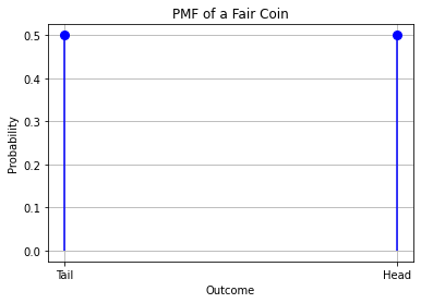
6.13.1.1. Example: Probability Mass Function for a Fair Coin#
A probability mass function can be plotted as a 2D diagram where the values of the function (\(P(x)\)) is plotted against the values of the independent variable \(x\). This is the diagram associated to the PMF of the previous example, where \(P(head) = P(tail) = 0.5\).
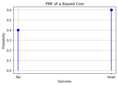
6.13.1.2. Example: Probability Mass Function for a Biased Coin#
Now suppose we tossed our coin for 10000 times and discovered that 6000 times the outcome was “head”, whereas 4000 times it was “tail”. We deduce the coin is not fair.
Using a frequentist approach, we can manually assign values to our PMF using the general formula:
That is, in our case:
We shall note that the probability we just defined satisfies all properties of probabilities, i.e.:
\(0 \leq P(x) \leq 1\ \forall x\)
\(\sum_{x}^{}{P(x) = 1}.\)
6.13.1.3. Exercise: Probability Mass Function#
Let \(X\) be a random variable representing the outcome of rolling a fair dice with \(6\) faces:
What is the space of possible values of \(X\)?
What is its cardinality?
What is the associated probability mass function \(P(X)\)?
Suppose the dice is not fair and \(P(X = 1) = 0.2\), whereas all other outcomes are equally probable. What is the probability mass function of \(P(X)\)?
Draw the PMF obtained for the dice.
6.13.2. Probability Density Functions (PDF) - Continuous Variables#
Probability distributions are called “probability density functions” when the random variable is continuous.
To be a probability density function over a variable \(X\), a function \(f:\Omega \rightarrow \lbrack 0,1\rbrack\) must satisfy the following properties:
The domain of \(f\) is the set of all possible values of \(X\).
\(\forall x \in \Omega,\ P(x) \geq 0\). No probability can be negative.
\(\int f(x)dx = 1\). This is equivalent to \(\sum P(x) = 1\) in the case of a discrete variable. The sum turns into an integral in the case of continuous variables.
Note that, in the case of continuous variables, we have:
NOTE: In general, we say that the density function at a given value \(x\) is zero: \(f(x)=0\). While this may seem counter-intuitive, we should consider the density function as the limit fo the probability as we narrow a neighborhood around \(x\). If the neighborhood has size \(0\), then the density will be zero. In practice, if we take a neighborhood which is non-zero, then we get an integral between two values and a final probability not equal to zero.
After all, from an intuitive point of view, the probability of having a value exactly equal to \(x\) is indeed zero, in the case of a continuous variable! So we should be more interested in the probability in a given range of values.
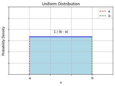
6.13.2.1. Example: Uniform PDF#
Let us consider a random number generator which outputs numbers comprised between \(a\) and \(b\).
Let \(X\) be a random variable assuming the values generated by the random number generator.
The PDF of \(X\) will be a uniform distribution such that:
\(P(x) = 0\ \forall x < a\ \ or\ x > b\);
\(P(x) = \frac{1}{b - a}\ \forall a \leq x \leq b\);
We can see that this PDF satisfies all constraints:
\(P(x) \geq 0\ \forall x.\)
\(\int P(x)dx = 1\) (prove that this is true as an exercise).
The diagram below shows an illustration of a uniform PDF with bounds a and b, i.e., \(U(a,b)\). Of course, continuous distributions can be (and generally are) much more complicated than that.
6.13.2.2. Cumulative Distribution Functions (CDF)#
Similar to the Empirical Cumulative Distribution Functions, we can define Cumulative Distribution Functions for random variables, starting from the density or mass functions. A cumulative distribution function is generally defined as:
6.13.2.3. CDF of Continuous Random Variables#
In the case of continuous random variables, the definition leads to:
The CDF is useful in different ways. For instance, it’s easy to see that:
6.13.2.4. Example#
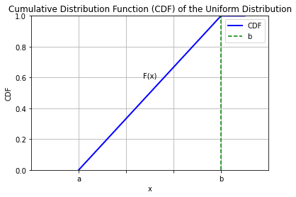
The CDF of the uniform distribution will be given by:
\(F(x) = 0\) for \(x < a\)
\(F(x) = \frac{x - a}{b - a}\) for \(a \leq x \leq b\)
\(F(x) = 1\) for \(x > b\)
The plot below shows a diagram:
6.13.2.5. CDF of Discrete Random Variables#
In the case of discrete random variables, the definition of CDF leads to:
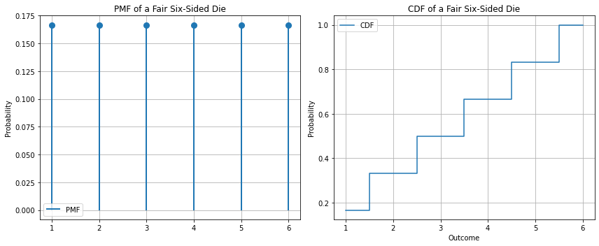
6.13.2.5.1. Example - PDF and CDF of a fair die#
In the case of a fair die, the PMF will be:
The CDF will be:
The diagram below shows an example:
6.13.3. Expectation#
When it is known that a random variable follows a probability distribution, it is possible to characterize that variable (and hence the related probability distribution) with some statistics.
The most straightforward of them is the expectation. The concept of expectation is very related to the concept of mean. When we compute the mean of a given set of numbers, we usually sum all the numbers together and then divide by the total.
Since a probability distribution will tell us which values will be more frequent than others, we can compute this mean with a weighted average, where the weights are given by the probability distribution.
Specifically, we can define the expectation of a random variable X as follows:
In the case of continuous variables, the expectation takes the form of an integral:
This is very related to the concept of mean value (or expected value) of a random variable.
6.13.4. Variance#
The variance gives a measure of how much variability there is in a variable \(X\) around its mean \(E\lbrack X\rbrack\).
The variance is defined as follows:
6.13.5. Covariance#
The covariance gives a measure of how two variables are linearly related to each other. It allows to measure to what extent the increase of one of the variables corresponds to an increase of the value of the other one.
Given two random variables \(X\) and \(Y\), the covariance is defined as follows:
We can distinguish the following terms:
\(E\lbrack X\rbrack\) and \(E\lbrack Y\rbrack\) are the expectations of \(X\) and \(Y.\)
\((X - E\lbrack X\rbrack)\) and \((Y - E\lbrack Y\rbrack)\) are the differences between the samples and the expected values.
\(\left( X - E\lbrack X\rbrack \right)\left( Y - E\lbrack Y\rbrack \right)\) computes the product between the differences.
We have:
If the signs of the terms agree, the product is positive.
If the signs of the terms disagree, the product is negative.
In practice, if when \(X\) is larger than the mean, then \(Y\) is larger than the mean and vice versa, when \(X\) is lower than the mean then \(Y\) is lower than the mean, then the two variables are correlated, and the covariance is high.
If \(X\) is a multi-dimensional variable \(X = \lbrack X_{1},X_{2},\ldots,X_{n}\rbrack\), we can compute all the possible covariances between variable pairs: \(Cov\lbrack X_{i},X_{j}\rbrack\). This allows to create a matrix, which is generally referred to as the covariance matrix. The general term of the covariance matrix \(Cov(X)\) is given by:
6.13.6. Standardization#
Similar to z-scoring, standardization transforms a random variable \(X\) into a variable \(Z\) so that it has:
Expectation equal to zero: \(E(X) = 0\).
Variance equal to one: \(Var(X) = 1\).
The new standardized variable will be:
6.14. References#
Parts of chapter 1 of [1];
Most of chapter 3 of [2];
Parts of chapters 5-7 of [3].
[1] Bishop, Christopher M. Pattern recognition and machine learning. springer, 2006. https://www.microsoft.com/en-us/research/uploads/prod/2006/01/Bishop-Pattern-Recognition-and-Machine-Learning-2006.pdf
[2] Goodfellow, Ian, Yoshua Bengio, and Aaron Courville. Deep learning. MIT press, 2016. https://www.deeplearningbook.org/
[3] Heumann, Christian, and Michael Schomaker Shalabh. Introduction to statistics and data analysis. Springer International Publishing Switzerland, 2016.