31. Laboratorio su Regressione Lineare#
La regressione lineare ci permette di modellare la relazione tra una variabile dipendente \(y\) e una o più variabili indipendenti (o regressori) \(x_i\). Ciò avviene definendo il seguente modello parametrico:
dove:
\(\beta_0, \ldots, \beta_n\) sono i parametri del modello;
\(\beta_0\) è l’intercetta;
\(\beta_1, \ldots, \beta_n\) sono detti coefficienti di regressione;
\(n\) è il numero di variabili indipendenti \(x_i\);
\(\epsilon\) è il termine di errore (o rumore), ovvero la parte di \(y\) che la regressione “non riesce a spiegare”.
Dato un insieme di dati, è possibile stimare i parametri ottimali \(\beta_0\) e \(\mathbf{\beta}\) del regressore lineare mediante una procedura di ottimizzazione. Il regressore calcolato fornisce un modello in grado di spiegare le relazioni (lineari) tra le variabili indipendenti e la variabile dipendente.
Inizieremo considerando il solito height-weight dataset:
import pandas as pd
data=pd.read_csv('http://antoninofurnari.it/downloads/height_weight.csv')
data.info()
data.head()
<class 'pandas.core.frame.DataFrame'>
RangeIndex: 4231 entries, 0 to 4230
Data columns (total 4 columns):
 #   Column  Non-Null Count  Dtype
---  ------  --------------  -----
 0   sex     4231 non-null   object
 1   BMI     4231 non-null   float64
 2   height  4231 non-null   float64
 3   weight  4231 non-null   float64
dtypes: float64(3), object(1)
memory usage: 132.3+ KB
| sex | BMI | height | weight | |
|---|---|---|---|---|
| 0 | M | 33.36 | 187.96 | 117.933920 |
| 1 | M | 26.54 | 177.80 | 83.914520 |
| 2 | F | 32.13 | 154.94 | 77.110640 |
| 3 | M | 26.62 | 172.72 | 79.378600 |
| 4 | F | 27.13 | 167.64 | 76.203456 |
31.1. Regressione Lineare Semplice#
Vediamo un esempio di regressione semplice (ovvero rispetto a una sola variabile indipendente \(x_1\)). Consideriamo le variabili weight e BMI, cercando di prevedere i valori di BMI da weight. Costruiremo dunque un modello lineare di questo tipo:
dove:
weight è la variabile indipendente;
BMI è la variabile dipendente;
\(\beta_1\) è il coefficiente di
weight;\(\beta_0\) è l’intercetta.
Per definire e calcolare il modello di regressione lineare, utilizzeremo il metodo dei minimi quadrati (Ordinary Least Squares - OLS), implementato dalla libreria statsmodels:
from statsmodels.formula.api import ols
#la notazione y ~ x indica che y è la variabile
#dipendente e x è la variabile indipendente
#le altre variabili del dataframe saranno scartate
model = ols("BMI ~ weight",data).fit()

#visualizziamo i parametri del modello
model.params
Intercept    7.371959
weight       0.252028
dtype: float64
Abbiamo calcolato il modello lineare:
che ci permette di calcolare il valore di BMI dai valori di weight.
🙋♂️ Domanda 1
Secondo il modello lineare trovato, che valore di BMI ha un soggetto che pesa 69 Kg? E per un soggetto che pesa 90 Kg?
Il modello mette a disposizione il metodo predict per effettuare questo tipo di calcoli. Il metodo però vuole che specifichiamo il nome delle variabili indipendenti per le quali stiamo fornendo i valori. Ciò si può fare definendo al volo un dizionario:
model.predict({'weight':[69, 90]})
0    24.761904
1    30.054496
dtype: float64
Il modello calcolato non è altro che una retta che fa corrispondere valori di weight a valori di BMI. Possiamo facilmente visualizzare la retta utilizzando la libreria seaborn:
import seaborn as sns
from matplotlib import pyplot as plt
sns.regplot(x='BMI',y='weight',data=data)
plt.show()
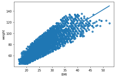
🙋♂️ Domanda 2
Cosa possiamo dire della retta visualizzata? Esistono valori per i quali l’errore commesso è maggiore? Qual è l’equazione della retta mostrata nel grafico?
31.1.1. Analisi di un regressore lineare semplice#
Analizziamo adesso il regrssore ottenuto e vediamo che interpretazione hanno i parametri individuati. Possiamo visualizzare un sommario sul regressore mediante il metodo summary dell’oggetto ols:
model.summary()
| Dep. Variable: | BMI | R-squared: | 0.704 |
|---|---|---|---|
| Model: | OLS | Adj. R-squared: | 0.704 |
| Method: | Least Squares | F-statistic: | 1.006e+04 |
| Date: | Tue, 31 Oct 2023 | Prob (F-statistic): | 0.00 |
| Time: | 06:41:15 | Log-Likelihood: | -10476. |
| No. Observations: | 4231 | AIC: | 2.096e+04 |
| Df Residuals: | 4229 | BIC: | 2.097e+04 |
| Df Model: | 1 | ||
| Covariance Type: | nonrobust |
| coef | std err | t | P>|t| | [0.025 | 0.975] | |
|---|---|---|---|---|---|---|
| Intercept | 7.3720 | 0.203 | 36.253 | 0.000 | 6.973 | 7.771 |
| weight | 0.2520 | 0.003 | 100.290 | 0.000 | 0.247 | 0.257 |
| Omnibus: | 342.463 | Durbin-Watson: | 2.007 |
|---|---|---|---|
| Prob(Omnibus): | 0.000 | Jarque-Bera (JB): | 467.107 |
| Skew: | 0.679 | Prob(JB): | 3.71e-102 |
| Kurtosis: | 3.896 | Cond. No. | 372. |
Notes:
[1] Standard Errors assume that the covariance matrix of the errors is correctly specified.
Il sommario presenta molte informazioni. Alcune di esse sono autoesplicative, come ad esempio “Dep. Variable”, “Model”, “Method”, “Date”, “Time”, “No. Observations”, “coef”. Altre sono invece molto specifiche. Tra tutti i valori mostrati, alcuni importanti sono:
R-squared e Adjusted R-squared;
F-statistic e prob(F-statistic);
Valori \(t\) dei singoli parametri e relativi valori di \(P>|t|\) (p-value);
I valori trovati per i singoli parametri. Analizziamo il significato di ciascuno di questi valori:
Il valore di \(R^2\) indica che la conoscenza di weight permette di ridurre l’errore sulle predizioni di BMI del \(70\%\). Ciò vuol dire che, benché weight da sola non riesca a spiegare (linearmente) BMI, le due variabili sono piuttosto correlate. (Si noti che in realtà sappiamo che BMI si calcola a partire da height e weight, quindi questa non dovrebbe essere una scoperta sorprendente). Il valore della F-statistic è alto, mentre quello di Prob(F-statistic) è nullo. Possiamo concludere che il regressore è statisticamente significativo.
I p-value relativi a entrambi i parametri sono nulli, pertanto entrambi i parametri sono statisticamente rilevanti. Il valore dell’intercetta è pari a \(7.38\). Ciò indica che a un peso di \(0\ Kg\) corrisponde un BMI pari a \(7.38\) secondo il modello trovato. Il valore del coefficiente di weight è pari a \(0.25\). Ciò significa che incrementando il peso di un kilogrammo, il BMI aumenta di \(0.25\ Kg/m^2\).
31.2. Regressione Lineare Multipla#
Vediamo adesso un esempio di regressione multipla. La regressione lineare multipla permette di studiare le relazioni tra una variabile dipendente e un insieme di variabili indipendenti. Calcoliamo un regressore lineare per predire i valori di BMI da quelli di height e weight:
model = ols('BMI ~ height + weight',data).fit()
model.summary()
| Dep. Variable: | BMI | R-squared: | 0.986 |
|---|---|---|---|
| Model: | OLS | Adj. R-squared: | 0.986 |
| Method: | Least Squares | F-statistic: | 1.513e+05 |
| Date: | Fri, 26 Oct 2018 | Prob (F-statistic): | 0.00 |
| Time: | 19:48:28 | Log-Likelihood: | -3987.0 |
| No. Observations: | 4231 | AIC: | 7980. |
| Df Residuals: | 4228 | BIC: | 7999. |
| Df Model: | 2 | ||
| Covariance Type: | nonrobust |
| coef | std err | t | P>|t| | [0.025 | 0.975] | |
|---|---|---|---|---|---|---|
| Intercept | 55.8865 | 0.171 | 327.627 | 0.000 | 55.552 | 56.221 |
| height | -0.3310 | 0.001 | -294.311 | 0.000 | -0.333 | -0.329 |
| weight | 0.3497 | 0.001 | 550.104 | 0.000 | 0.348 | 0.351 |
| Omnibus: | 441.026 | Durbin-Watson: | 1.980 |
|---|---|---|---|
| Prob(Omnibus): | 0.000 | Jarque-Bera (JB): | 3489.395 |
| Skew: | 0.132 | Prob(JB): | 0.00 |
| Kurtosis: | 7.441 | Cond. No. | 3.36e+03 |
Warnings:
[1] Standard Errors assume that the covariance matrix of the errors is correctly specified.
[2] The condition number is large, 3.36e+03. This might indicate that there are
strong multicollinearity or other numerical problems.
Il regressore lineare trovato ha un valore di \(R^2\) molto alto (\(0.986\)), una F-statistic alta e un valore di Prob(F-statistic) nullo. Possiamo concludere che il regressore è significativo. I p-value dei parametri sono tutti nulli, il che significa che le variabili contribuiscono tutte significativamente alla regressione.
L’intercetta ha un valore pari a \(55.88\), il che indica che, idealmente, un soggetto di peso e altezza nulla avrebbe un BMI pari a \(55.88\ Kg/m^2\). Il coefficiente di height indica che quando l’altezza viene incrementata di un metro, il BMI viene decrementato di \(0.33\ Kg/m^2\). Analogamente, quando il peso viene incrementato di un kilogrammo, il BMI viene incrementato di \(0.35\ Kg/m^2\).
31.2.1. Boston House Pricing Dataset#
Vediamo adesso un esempio con un dataset più complesso. Utilizzeremo il dataset “Boston” che contiene osservazioni relativi ai prezzi di diverse case nei sobborghi di Boston. Carichiamo il dataset mediante la funzione get_rdataset di statsmodels, che permette di caricare dataset contenuti nelle librerie del linguaggio R:
from statsmodels.datasets import get_rdataset
boston = get_rdataset('Boston', package='MASS')
I dataset caricati mediante get_rdataset presentano la medesima struttura. Esiste una documentazione nella proprietà __doc__. Stampiamola per farci un’idea più precisa sul dataset:
print(boston.__doc__)
.. container::

   ====== ===============
   Boston R Documentation
   ====== ===============

   .. rubric:: Housing Values in Suburbs of Boston
      :name: Boston

   .. rubric:: Description
      :name: description

   The ``Boston`` data frame has 506 rows and 14 columns.

   .. rubric:: Usage
      :name: usage

   .. code:: R

      Boston

   .. rubric:: Format
      :name: format

   This data frame contains the following columns:

   ``crim``
      per capita crime rate by town.

   ``zn``
      proportion of residential land zoned for lots over 25,000 sq.ft.

   ``indus``
      proportion of non-retail business acres per town.

   ``chas``
      Charles River dummy variable (= 1 if tract bounds river; 0
      otherwise).

   ``nox``
      nitrogen oxides concentration (parts per 10 million).

   ``rm``
      average number of rooms per dwelling.

   ``age``
      proportion of owner-occupied units built prior to 1940.

   ``dis``
      weighted mean of distances to five Boston employment centres.

   ``rad``
      index of accessibility to radial highways.

   ``tax``
      full-value property-tax rate per $10,000.

   ``ptratio``
      pupil-teacher ratio by town.

   ``black``
      ``1000(Bk - 0.63)^2`` where ``Bk`` is the proportion of blacks by
      town.

   ``lstat``
      lower status of the population (percent).

   ``medv``
      median value of owner-occupied homes in $1000s.

   .. rubric:: Source
      :name: source

   Harrison, D. and Rubinfeld, D.L. (1978) Hedonic prices and the demand
   for clean air. *J. Environ. Economics and Management* **5**, 81–102.

   Belsley D.A., Kuh, E. and Welsch, R.E. (1980) *Regression
   Diagnostics. Identifying Influential Data and Sources of
   Collinearity.* New York: Wiley.
Il dataframe contenente le osservazioni si trova all’interno della proprietà data:
boston.data.head()
| crim | zn | indus | chas | nox | rm | age | dis | rad | tax | ptratio | black | lstat | medv | |
|---|---|---|---|---|---|---|---|---|---|---|---|---|---|---|
| 0 | 0.00632 | 18.0 | 2.31 | 0 | 0.538 | 6.575 | 65.2 | 4.0900 | 1 | 296 | 15.3 | 396.90 | 4.98 | 24.0 |
| 1 | 0.02731 | 0.0 | 7.07 | 0 | 0.469 | 6.421 | 78.9 | 4.9671 | 2 | 242 | 17.8 | 396.90 | 9.14 | 21.6 |
| 2 | 0.02729 | 0.0 | 7.07 | 0 | 0.469 | 7.185 | 61.1 | 4.9671 | 2 | 242 | 17.8 | 392.83 | 4.03 | 34.7 |
| 3 | 0.03237 | 0.0 | 2.18 | 0 | 0.458 | 6.998 | 45.8 | 6.0622 | 3 | 222 | 18.7 | 394.63 | 2.94 | 33.4 |
| 4 | 0.06905 | 0.0 | 2.18 | 0 | 0.458 | 7.147 | 54.2 | 6.0622 | 3 | 222 | 18.7 | 396.90 | 5.33 | 36.2 |
Questo dataset è generalmente utilizzato come un dataset di regressione, nel quale l’obiettivo è quello di predire il valore di medv (prezzo medio delle case in migliaia di dollari) a partire dai valori delle altre variabili.
31.2.2. Regressori lineari, variabili categoriche e variabili dummy#
Notiamo che le variabili rad e chas sono categoriche. Quando si lavora con regressori lineari e variabili categoriche bisogna fare attenzione:
Le variabili categoriche non vanno utilizzate come variabili dipendenti di un regressore lineare;
Le variabili categoriche possono essere utilizzate invece come variabili indipendenti solo se binarie.
chasè binaria, quindi possiamo includerla tra le variabili indipendenti.radinvece non è binaria, pertanto non può essere inclusa tra le variabili per la regressione.
Se vogliamo includere rad tra le variabili per la regressione lineare, dobbiamo trasformarla in un insiem di variabili binarie “dummy”. Ogni variabile “dummy” indicherà per ogni osservazione, se essa appartiene a una specifica classe tra quelle della variabile categorica considerata.
Vediamo un esempio:
var = pd.Series(['A','A','B','A','C','C','B','A','C','B'])
var
0    A
1    A
2    B
3    A
4    C
5    C
6    B
7    A
8    C
9    B
dtype: object
Si consideri var come una variabile categorica che consta di \(10\) osservazioni e \(3\) classi. Possiamo sostituire la variabile var con tre variabili A,B,C tali che A sarà pari a \(1\) solo quando var è uguale ad A, C sarà pari a \(1\) solo quando var è uguale ad C. Possiamo ottenere queste tre variabili dummy mediante la funzione get_dummies di Pandas:
pd.get_dummies(var)
| A | B | C | |
|---|---|---|---|
| 0 | 1 | 0 | 0 |
| 1 | 1 | 0 | 0 |
| 2 | 0 | 1 | 0 |
| 3 | 1 | 0 | 0 |
| 4 | 0 | 0 | 1 |
| 5 | 0 | 0 | 1 |
| 6 | 0 | 1 | 0 |
| 7 | 1 | 0 | 0 |
| 8 | 0 | 0 | 1 |
| 9 | 0 | 1 | 0 |
Confrontiamo ad esempio l’osservazione di indice \(5\) della serie e del DataFrame di variabili dummy:
print(var[5],'\n')
print(pd.get_dummies(var).loc[5])
C

A    0
B    0
C    1
Name: 5, dtype: uint8
Il valore di var è \(5\). In maniera corrispondente, la variabile dummy C è pari a \(1\), mentre le altre sono pari a zero. Questo tipo di rappresentazione di var è tuttavia ridondante. Infatti, se sappiamo che \(B=0\) e \(C=0\), possiamo facilmente dedurre che \(A=1\). Questa semplice ridondanza può creare problemi di clacolo numerico nell’ottimizzazione del regressore lineare. Per evitarla, generalmente si esclude una delle variabili dummy. Possiamo ottenere questo risultato come segue:
pd.get_dummies(var,drop_first=True)
| B | C | |
|---|---|---|
| 0 | 0 | 0 |
| 1 | 0 | 0 |
| 2 | 1 | 0 |
| 3 | 0 | 0 |
| 4 | 0 | 1 |
| 5 | 0 | 1 |
| 6 | 1 | 0 |
| 7 | 0 | 0 |
| 8 | 0 | 1 |
| 9 | 1 | 0 |
Possiamo convertire la variabile categorica rad in un insieme di variabili dummy come segue:
boston_mod=pd.get_dummies(boston.data, columns=['rad'],drop_first=True)
boston_mod.head()
| crim | zn | indus | chas | nox | rm | age | dis | tax | ptratio | ... | lstat | medv | rad_2 | rad_3 | rad_4 | rad_5 | rad_6 | rad_7 | rad_8 | rad_24 | |
|---|---|---|---|---|---|---|---|---|---|---|---|---|---|---|---|---|---|---|---|---|---|
| 0 | 0.00632 | 18.0 | 2.31 | 0 | 0.538 | 6.575 | 65.2 | 4.0900 | 296 | 15.3 | ... | 4.98 | 24.0 | 0 | 0 | 0 | 0 | 0 | 0 | 0 | 0 |
| 1 | 0.02731 | 0.0 | 7.07 | 0 | 0.469 | 6.421 | 78.9 | 4.9671 | 242 | 17.8 | ... | 9.14 | 21.6 | 1 | 0 | 0 | 0 | 0 | 0 | 0 | 0 |
| 2 | 0.02729 | 0.0 | 7.07 | 0 | 0.469 | 7.185 | 61.1 | 4.9671 | 242 | 17.8 | ... | 4.03 | 34.7 | 1 | 0 | 0 | 0 | 0 | 0 | 0 | 0 |
| 3 | 0.03237 | 0.0 | 2.18 | 0 | 0.458 | 6.998 | 45.8 | 6.0622 | 222 | 18.7 | ... | 2.94 | 33.4 | 0 | 1 | 0 | 0 | 0 | 0 | 0 | 0 |
| 4 | 0.06905 | 0.0 | 2.18 | 0 | 0.458 | 7.147 | 54.2 | 6.0622 | 222 | 18.7 | ... | 5.33 | 36.2 | 0 | 1 | 0 | 0 | 0 | 0 | 0 | 0 |
5 rows × 21 columns
Ispezioniamo i nomi delle colonne:
boston_mod.columns
Index(['crim', 'zn', 'indus', 'chas', 'nox', 'rm', 'age', 'dis', 'tax',
       'ptratio', 'black', 'lstat', 'medv', 'rad_2', 'rad_3', 'rad_4', 'rad_5',
       'rad_6', 'rad_7', 'rad_8', 'rad_24'],
      dtype='object')
Notiamo che rad è stata rimossa e sostituita da diverse variabili dummy, rappresentanti i vari valori assunti da rad. Possiamo adesso procedere al calcolo del regressore lineare multiplo:
model=ols("""medv ~ crim + zn + indus + chas + nox + rm +age + dis + tax +
          ptratio + black + lstat + rad_2 + rad_3 + rad_4 + rad_5 + rad_6 +
          rad_7 + rad_8 + rad_24""", boston_mod).fit()
model.summary()
| Dep. Variable: | medv | R-squared: | 0.750 |
|---|---|---|---|
| Model: | OLS | Adj. R-squared: | 0.740 |
| Method: | Least Squares | F-statistic: | 72.70 |
| Date: | Tue, 31 Oct 2023 | Prob (F-statistic): | 8.29e-132 |
| Time: | 06:43:47 | Log-Likelihood: | -1489.6 |
| No. Observations: | 506 | AIC: | 3021. |
| Df Residuals: | 485 | BIC: | 3110. |
| Df Model: | 20 | ||
| Covariance Type: | nonrobust |
| coef | std err | t | P>|t| | [0.025 | 0.975] | |
|---|---|---|---|---|---|---|
| Intercept | 35.2596 | 5.434 | 6.489 | 0.000 | 24.583 | 45.936 |
| crim | -0.1088 | 0.033 | -3.329 | 0.001 | -0.173 | -0.045 |
| zn | 0.0549 | 0.014 | 3.880 | 0.000 | 0.027 | 0.083 |
| indus | 0.0238 | 0.064 | 0.373 | 0.709 | -0.101 | 0.149 |
| chas | 2.5242 | 0.863 | 2.924 | 0.004 | 0.828 | 4.220 |
| nox | -17.5731 | 3.896 | -4.510 | 0.000 | -25.229 | -9.917 |
| rm | 3.6655 | 0.421 | 8.703 | 0.000 | 2.838 | 4.493 |
| age | 0.0005 | 0.013 | 0.035 | 0.972 | -0.026 | 0.026 |
| dis | -1.5545 | 0.202 | -7.699 | 0.000 | -1.951 | -1.158 |
| tax | -0.0087 | 0.004 | -2.246 | 0.025 | -0.016 | -0.001 |
| ptratio | -0.9724 | 0.144 | -6.731 | 0.000 | -1.256 | -0.689 |
| black | 0.0094 | 0.003 | 3.531 | 0.000 | 0.004 | 0.015 |
| lstat | -0.5292 | 0.051 | -10.451 | 0.000 | -0.629 | -0.430 |
| rad_2 | 1.4889 | 1.478 | 1.008 | 0.314 | -1.414 | 4.392 |
| rad_3 | 4.6813 | 1.335 | 3.506 | 0.000 | 2.058 | 7.305 |
| rad_4 | 2.5762 | 1.187 | 2.170 | 0.031 | 0.243 | 4.909 |
| rad_5 | 2.9185 | 1.208 | 2.417 | 0.016 | 0.546 | 5.291 |
| rad_6 | 1.1858 | 1.464 | 0.810 | 0.418 | -1.691 | 4.062 |
| rad_7 | 4.8790 | 1.571 | 3.105 | 0.002 | 1.792 | 7.966 |
| rad_8 | 4.8398 | 1.492 | 3.245 | 0.001 | 1.909 | 7.771 |
| rad_24 | 7.4617 | 1.789 | 4.172 | 0.000 | 3.947 | 10.976 |
| Omnibus: | 183.890 | Durbin-Watson: | 1.089 |
|---|---|---|---|
| Prob(Omnibus): | 0.000 | Jarque-Bera (JB): | 858.805 |
| Skew: | 1.554 | Prob(JB): | 3.26e-187 |
| Kurtosis: | 8.575 | Cond. No. | 1.60e+04 |
Notes:
[1] Standard Errors assume that the covariance matrix of the errors is correctly specified.
[2] The condition number is large, 1.6e+04. This might indicate that there are
strong multicollinearity or other numerical problems.
Il regressore ottenuto presenta un valore di \(R^2\) piuttosto alto. Ciò vuol dire che, globalmente, le variabili indipendenti sono correlate con la variabile dipendente. La F-statistic è alta e il p-value corrispondente è molto basso. Il regressore è, globalmente, statisticamente significativo.
Passiamo all’analisi dei p-value dei singoli parametri trovati. I p-value delle seguenti variabili sono più alti di \(0.05\):
indus;age;rad2;rad6.
Queste variabili non contribuiscono significativamente alla regressione. Analizziamo i valori dei parametri relativi a varabili che contribuiscono statisticamente alla regressione:
intercept: quando tutte le altre variabili assumono valori nulli,medvassume il valore \(35.26\). Ricordiamo chemedvesprime il prezzo medio delle case in migliaia di dollari, per cui il “prezzo medio base” delle case è di circa \(35260\) dollari;crim: l’incremento di una unità del tasso di criminalità pro-capite abbassa il valore delle case di cica \(108\) dollari;zn: l’incremento di una unità della proporzione di terre destinate a uso residenziale aumenta il valore delle case di circa \(54\) dollari;chas: quando la variabile è pari a \(1\) (ricordiamo che si tratta di una variabile categorica), il prezzo delle case sale di circa \(2500\) dollari. Possiamo dire che le case vicine al fiume tendono ad essere più care;nox: l’aumento di una unità della concentrazione di ossido di azoto abbassa i prezzi delle case di circa \(17500\) dollari. Questo può sembrare un numero altissimo, ma si noti che i valori dinoxvariano tra un minimo di \(0.38\) a un massimo di \(0.87\), per cui non si verificheranno decrementi dei prezzi delle case così grandi;rm: l’incremento del numero di stanze di una unità incrementa il prezzo della casa di circa \(3600\) dollari;dis: l’incremento di una unità della distanza media dal centro diminuisce il prezzo delle case di circa \(1500\) dollari (le case più distanti dal centro valgono di meno);tax: l’aumento di un unità del tax-rate della proprietà ne diminuisce il valore di 8 dollari. Sembra un decremento trascurabile, tuttavia, si consideri che il range ditaxè compreso tra \(187\) e \(711\);ptratio: l’aumento di una unità del rapporto insegnante-alunni diminuisce il valore della proprietà di circa \(1000\) dollari;black: l’aumento di una unità del valore diblack(una variabile dipendente dalla proporzione tra abitanti bianchi e neri) incrementa il valore delle case di pochi dollari. Si consideri che il range diblackva da circa \(0\) a \(396\);lstat: l’aumento di una unità del valore di questa variabile (percenutale di abitanti meno abbienti) diminuisce il prezzo delle case di circa \(500\) dollari;I coefficienti appresi per le variabili dummy di
radindicano che quandoradassume il valore 24, il valore delle case aumenta di circa \(7500\) dollari. Altri valori diradcontribuiscono differentemente all’incremento del valore dimedv;
🙋♂️ Domanda 3
Dati i risultati del regressore lineare, qual è la variabile più influente nella regressione?
model=ols("""medv ~ crim + zn + indus + chas + nox + rm +age + dis + tax +
          ptratio + black + lstat + rad""", boston.data).fit()
model.summary()
| Dep. Variable: | medv | R-squared: | 0.741 |
|---|---|---|---|
| Model: | OLS | Adj. R-squared: | 0.734 |
| Method: | Least Squares | F-statistic: | 108.1 |
| Date: | Tue, 31 Oct 2023 | Prob (F-statistic): | 6.72e-135 |
| Time: | 06:48:40 | Log-Likelihood: | -1498.8 |
| No. Observations: | 506 | AIC: | 3026. |
| Df Residuals: | 492 | BIC: | 3085. |
| Df Model: | 13 | ||
| Covariance Type: | nonrobust |
| coef | std err | t | P>|t| | [0.025 | 0.975] | |
|---|---|---|---|---|---|---|
| Intercept | 36.4595 | 5.103 | 7.144 | 0.000 | 26.432 | 46.487 |
| crim | -0.1080 | 0.033 | -3.287 | 0.001 | -0.173 | -0.043 |
| zn | 0.0464 | 0.014 | 3.382 | 0.001 | 0.019 | 0.073 |
| indus | 0.0206 | 0.061 | 0.334 | 0.738 | -0.100 | 0.141 |
| chas | 2.6867 | 0.862 | 3.118 | 0.002 | 0.994 | 4.380 |
| nox | -17.7666 | 3.820 | -4.651 | 0.000 | -25.272 | -10.262 |
| rm | 3.8099 | 0.418 | 9.116 | 0.000 | 2.989 | 4.631 |
| age | 0.0007 | 0.013 | 0.052 | 0.958 | -0.025 | 0.027 |
| dis | -1.4756 | 0.199 | -7.398 | 0.000 | -1.867 | -1.084 |
| tax | -0.0123 | 0.004 | -3.280 | 0.001 | -0.020 | -0.005 |
| ptratio | -0.9527 | 0.131 | -7.283 | 0.000 | -1.210 | -0.696 |
| black | 0.0093 | 0.003 | 3.467 | 0.001 | 0.004 | 0.015 |
| lstat | -0.5248 | 0.051 | -10.347 | 0.000 | -0.624 | -0.425 |
| rad | 0.3060 | 0.066 | 4.613 | 0.000 | 0.176 | 0.436 |
| Omnibus: | 178.041 | Durbin-Watson: | 1.078 |
|---|---|---|---|
| Prob(Omnibus): | 0.000 | Jarque-Bera (JB): | 783.126 |
| Skew: | 1.521 | Prob(JB): | 8.84e-171 |
| Kurtosis: | 8.281 | Cond. No. | 1.51e+04 |
Notes:
[1] Standard Errors assume that the covariance matrix of the errors is correctly specified.
[2] The condition number is large, 1.51e+04. This might indicate that there are
strong multicollinearity or other numerical problems.
It should be noted that, when it is obvious that a variable is categorical, statsmodels automatically create dummy variables internally. For instance, let us modify the dataframe so that rad becomes text:
boston2 = boston.data.copy()
boston2['rad'] = boston2['rad'].apply(str)
boston2['rad']
0      1
1      2
2      2
3      3
4      3
      ..
501    1
502    1
503    1
504    1
505    1
Name: rad, Length: 506, dtype: object
If we fit a linear regressor model on the modified dataset, statsmodels will introduce different dummy variables for the different values of rad:
model=ols("""medv ~ crim + zn + indus + chas + nox + rm +age + dis + tax +
          ptratio + black + lstat + rad""", boston2).fit()
model.summary()
| Dep. Variable: | medv | R-squared: | 0.750 |
|---|---|---|---|
| Model: | OLS | Adj. R-squared: | 0.740 |
| Method: | Least Squares | F-statistic: | 72.70 |
| Date: | Tue, 31 Oct 2023 | Prob (F-statistic): | 8.29e-132 |
| Time: | 06:57:15 | Log-Likelihood: | -1489.6 |
| No. Observations: | 506 | AIC: | 3021. |
| Df Residuals: | 485 | BIC: | 3110. |
| Df Model: | 20 | ||
| Covariance Type: | nonrobust |
| coef | std err | t | P>|t| | [0.025 | 0.975] | |
|---|---|---|---|---|---|---|
| Intercept | 35.2596 | 5.434 | 6.489 | 0.000 | 24.583 | 45.936 |
| rad[T.2] | 1.4889 | 1.478 | 1.008 | 0.314 | -1.414 | 4.392 |
| rad[T.24] | 7.4617 | 1.789 | 4.172 | 0.000 | 3.947 | 10.976 |
| rad[T.3] | 4.6813 | 1.335 | 3.506 | 0.000 | 2.058 | 7.305 |
| rad[T.4] | 2.5762 | 1.187 | 2.170 | 0.031 | 0.243 | 4.909 |
| rad[T.5] | 2.9185 | 1.208 | 2.417 | 0.016 | 0.546 | 5.291 |
| rad[T.6] | 1.1858 | 1.464 | 0.810 | 0.418 | -1.691 | 4.062 |
| rad[T.7] | 4.8790 | 1.571 | 3.105 | 0.002 | 1.792 | 7.966 |
| rad[T.8] | 4.8398 | 1.492 | 3.245 | 0.001 | 1.909 | 7.771 |
| crim | -0.1088 | 0.033 | -3.329 | 0.001 | -0.173 | -0.045 |
| zn | 0.0549 | 0.014 | 3.880 | 0.000 | 0.027 | 0.083 |
| indus | 0.0238 | 0.064 | 0.373 | 0.709 | -0.101 | 0.149 |
| chas | 2.5242 | 0.863 | 2.924 | 0.004 | 0.828 | 4.220 |
| nox | -17.5731 | 3.896 | -4.510 | 0.000 | -25.229 | -9.917 |
| rm | 3.6655 | 0.421 | 8.703 | 0.000 | 2.838 | 4.493 |
| age | 0.0005 | 0.013 | 0.035 | 0.972 | -0.026 | 0.026 |
| dis | -1.5545 | 0.202 | -7.699 | 0.000 | -1.951 | -1.158 |
| tax | -0.0087 | 0.004 | -2.246 | 0.025 | -0.016 | -0.001 |
| ptratio | -0.9724 | 0.144 | -6.731 | 0.000 | -1.256 | -0.689 |
| black | 0.0094 | 0.003 | 3.531 | 0.000 | 0.004 | 0.015 |
| lstat | -0.5292 | 0.051 | -10.451 | 0.000 | -0.629 | -0.430 |
| Omnibus: | 183.890 | Durbin-Watson: | 1.089 |
|---|---|---|---|
| Prob(Omnibus): | 0.000 | Jarque-Bera (JB): | 858.805 |
| Skew: | 1.554 | Prob(JB): | 3.26e-187 |
| Kurtosis: | 8.575 | Cond. No. | 1.60e+04 |
Notes:
[1] Standard Errors assume that the covariance matrix of the errors is correctly specified.
[2] The condition number is large, 1.6e+04. This might indicate that there are
strong multicollinearity or other numerical problems.
Alternatively, we can instruct statsmodels to use a variable as a categorical one with the C(variable) tag:
model=ols("""medv ~ crim + zn + indus + chas + nox + rm +age + dis + tax +
          ptratio + black + lstat + C(rad)""", boston.data).fit()
model.summary()
| Dep. Variable: | medv | R-squared: | 0.750 |
|---|---|---|---|
| Model: | OLS | Adj. R-squared: | 0.740 |
| Method: | Least Squares | F-statistic: | 72.70 |
| Date: | Tue, 31 Oct 2023 | Prob (F-statistic): | 8.29e-132 |
| Time: | 07:05:32 | Log-Likelihood: | -1489.6 |
| No. Observations: | 506 | AIC: | 3021. |
| Df Residuals: | 485 | BIC: | 3110. |
| Df Model: | 20 | ||
| Covariance Type: | nonrobust |
| coef | std err | t | P>|t| | [0.025 | 0.975] | |
|---|---|---|---|---|---|---|
| Intercept | 35.2596 | 5.434 | 6.489 | 0.000 | 24.583 | 45.936 |
| C(rad)[T.2] | 1.4889 | 1.478 | 1.008 | 0.314 | -1.414 | 4.392 |
| C(rad)[T.3] | 4.6813 | 1.335 | 3.506 | 0.000 | 2.058 | 7.305 |
| C(rad)[T.4] | 2.5762 | 1.187 | 2.170 | 0.031 | 0.243 | 4.909 |
| C(rad)[T.5] | 2.9185 | 1.208 | 2.417 | 0.016 | 0.546 | 5.291 |
| C(rad)[T.6] | 1.1858 | 1.464 | 0.810 | 0.418 | -1.691 | 4.062 |
| C(rad)[T.7] | 4.8790 | 1.571 | 3.105 | 0.002 | 1.792 | 7.966 |
| C(rad)[T.8] | 4.8398 | 1.492 | 3.245 | 0.001 | 1.909 | 7.771 |
| C(rad)[T.24] | 7.4617 | 1.789 | 4.172 | 0.000 | 3.947 | 10.976 |
| crim | -0.1088 | 0.033 | -3.329 | 0.001 | -0.173 | -0.045 |
| zn | 0.0549 | 0.014 | 3.880 | 0.000 | 0.027 | 0.083 |
| indus | 0.0238 | 0.064 | 0.373 | 0.709 | -0.101 | 0.149 |
| chas | 2.5242 | 0.863 | 2.924 | 0.004 | 0.828 | 4.220 |
| nox | -17.5731 | 3.896 | -4.510 | 0.000 | -25.229 | -9.917 |
| rm | 3.6655 | 0.421 | 8.703 | 0.000 | 2.838 | 4.493 |
| age | 0.0005 | 0.013 | 0.035 | 0.972 | -0.026 | 0.026 |
| dis | -1.5545 | 0.202 | -7.699 | 0.000 | -1.951 | -1.158 |
| tax | -0.0087 | 0.004 | -2.246 | 0.025 | -0.016 | -0.001 |
| ptratio | -0.9724 | 0.144 | -6.731 | 0.000 | -1.256 | -0.689 |
| black | 0.0094 | 0.003 | 3.531 | 0.000 | 0.004 | 0.015 |
| lstat | -0.5292 | 0.051 | -10.451 | 0.000 | -0.629 | -0.430 |
| Omnibus: | 183.890 | Durbin-Watson: | 1.089 |
|---|---|---|---|
| Prob(Omnibus): | 0.000 | Jarque-Bera (JB): | 858.805 |
| Skew: | 1.554 | Prob(JB): | 3.26e-187 |
| Kurtosis: | 8.575 | Cond. No. | 1.60e+04 |
Notes:
[1] Standard Errors assume that the covariance matrix of the errors is correctly specified.
[2] The condition number is large, 1.6e+04. This might indicate that there are
strong multicollinearity or other numerical problems.
ols("weight ~ BMI + height + sex",data).fit().summary()
| Dep. Variable: | weight | R-squared: | 0.990 |
|---|---|---|---|
| Model: | OLS | Adj. R-squared: | 0.990 |
| Method: | Least Squares | F-statistic: | 1.392e+05 |
| Date: | Tue, 31 Oct 2023 | Prob (F-statistic): | 0.00 |
| Time: | 06:54:01 | Log-Likelihood: | -8403.1 |
| No. Observations: | 4231 | AIC: | 1.681e+04 |
| Df Residuals: | 4227 | BIC: | 1.684e+04 |
| Df Model: | 3 | ||
| Covariance Type: | nonrobust |
| coef | std err | t | P>|t| | [0.025 | 0.975] | |
|---|---|---|---|---|---|---|
| Intercept | -158.3473 | 0.670 | -236.287 | 0.000 | -159.661 | -157.033 |
| sex[T.M] | 0.0592 | 0.079 | 0.753 | 0.451 | -0.095 | 0.213 |
| BMI | 2.8199 | 0.005 | 546.155 | 0.000 | 2.810 | 2.830 |
| height | 0.9440 | 0.004 | 240.347 | 0.000 | 0.936 | 0.952 |
| Omnibus: | 412.503 | Durbin-Watson: | 1.978 |
|---|---|---|---|
| Prob(Omnibus): | 0.000 | Jarque-Bera (JB): | 2913.710 |
| Skew: | 0.146 | Prob(JB): | 0.00 |
| Kurtosis: | 7.055 | Cond. No. | 4.27e+03 |
Notes:
[1] Standard Errors assume that the covariance matrix of the errors is correctly specified.
[2] The condition number is large, 4.27e+03. This might indicate that there are
strong multicollinearity or other numerical problems.
However, there is less control on which dummy variables to include or not in the model, as seen in the next section.
31.2.3. Backward Elimination#
Il modello di regressione lineare calcolato è in generale buono, ma include alcune variabili che non contribuiscono significativamente alla regressione. In pratica, queste variabili possono inficiare il calcolo del regressore lineare e quindi sarebbe ideale non averle dentro. Potremmo rimuoverle tutte, ma non siamo sicuri che, in assenza di alcune, le altre non acquisiscano una qualche significatività. Esistono diverse tecniche per eliminare tali variabili. Una delle possibilità consiste nell’usare il metodo della backward elimination, che è definito come segue:
Si calcola il regressore lineare considerando tutte le variabili dipendenti;
Se tutte le variabili sono significative, il regressore trovato è quello finale;
Se qualche variabile non è significativa, si rimuove la variabile con p-value più alto, si ricalcola il regressore lineare e si va al punto 2.
Alla fine del processo, otterremo un regressore in cui tutte le variabili sono significative.
Applichiamo il processo al nostro esempio. La variabile con p-value più alto è age. Riomuoviamola e ricalcoliamo il regressore:
model=ols("""medv ~ crim + zn + indus + chas + nox + rm + dis + tax +
          ptratio + black + lstat + rad_2 + rad_3 + rad_4 + rad_5 + rad_6 +
          rad_7 + rad_8 + rad_24""", boston_mod).fit()
model.summary()
| Dep. Variable: | medv | R-squared: | 0.750 |
|---|---|---|---|
| Model: | OLS | Adj. R-squared: | 0.740 |
| Method: | Least Squares | F-statistic: | 76.68 |
| Date: | Tue, 31 Oct 2023 | Prob (F-statistic): | 9.34e-133 |
| Time: | 06:44:13 | Log-Likelihood: | -1489.6 |
| No. Observations: | 506 | AIC: | 3019. |
| Df Residuals: | 486 | BIC: | 3104. |
| Df Model: | 19 | ||
| Covariance Type: | nonrobust |
| coef | std err | t | P>|t| | [0.025 | 0.975] | |
|---|---|---|---|---|---|---|
| Intercept | 35.2429 | 5.407 | 6.518 | 0.000 | 24.619 | 45.867 |
| crim | -0.1088 | 0.033 | -3.333 | 0.001 | -0.173 | -0.045 |
| zn | 0.0548 | 0.014 | 3.900 | 0.000 | 0.027 | 0.082 |
| indus | 0.0238 | 0.064 | 0.374 | 0.709 | -0.101 | 0.149 |
| chas | 2.5256 | 0.861 | 2.932 | 0.004 | 0.833 | 4.218 |
| nox | -17.5386 | 3.765 | -4.659 | 0.000 | -24.936 | -10.142 |
| rm | 3.6682 | 0.414 | 8.869 | 0.000 | 2.856 | 4.481 |
| dis | -1.5566 | 0.193 | -8.058 | 0.000 | -1.936 | -1.177 |
| tax | -0.0087 | 0.004 | -2.250 | 0.025 | -0.016 | -0.001 |
| ptratio | -0.9719 | 0.144 | -6.769 | 0.000 | -1.254 | -0.690 |
| black | 0.0094 | 0.003 | 3.544 | 0.000 | 0.004 | 0.015 |
| lstat | -0.5286 | 0.047 | -11.130 | 0.000 | -0.622 | -0.435 |
| rad_2 | 1.4910 | 1.475 | 1.011 | 0.313 | -1.407 | 4.389 |
| rad_3 | 4.6798 | 1.333 | 3.510 | 0.000 | 2.060 | 7.300 |
| rad_4 | 2.5748 | 1.185 | 2.172 | 0.030 | 0.246 | 4.904 |
| rad_5 | 2.9185 | 1.206 | 2.419 | 0.016 | 0.548 | 5.289 |
| rad_6 | 1.1833 | 1.461 | 0.810 | 0.418 | -1.687 | 4.053 |
| rad_7 | 4.8767 | 1.568 | 3.110 | 0.002 | 1.795 | 7.958 |
| rad_8 | 4.8423 | 1.488 | 3.253 | 0.001 | 1.918 | 7.767 |
| rad_24 | 7.4563 | 1.780 | 4.188 | 0.000 | 3.958 | 10.954 |
| Omnibus: | 184.084 | Durbin-Watson: | 1.088 |
|---|---|---|---|
| Prob(Omnibus): | 0.000 | Jarque-Bera (JB): | 861.138 |
| Skew: | 1.555 | Prob(JB): | 1.01e-187 |
| Kurtosis: | 8.583 | Cond. No. | 1.57e+04 |
Notes:
[1] Standard Errors assume that the covariance matrix of the errors is correctly specified.
[2] The condition number is large, 1.57e+04. This might indicate that there are
strong multicollinearity or other numerical problems.
Notiamo che il valore di \(R^2\) è rimasto invariato. Esistono ancora variabili non statisticamente rilevanti. Rimuoviamo indus, che ha il p-value più alto:
model=ols("""medv ~ crim + zn + chas + nox + rm + dis + tax +
          ptratio + black + lstat + rad_2 + rad_3 + rad_4 + rad_5 + rad_6 +
          rad_7 + rad_8 + rad_24""", boston_mod).fit()
model.summary()
| Dep. Variable: | medv | R-squared: | 0.750 |
|---|---|---|---|
| Model: | OLS | Adj. R-squared: | 0.741 |
| Method: | Least Squares | F-statistic: | 81.08 |
| Date: | Tue, 31 Oct 2023 | Prob (F-statistic): | 1.10e-133 |
| Time: | 06:44:17 | Log-Likelihood: | -1489.7 |
| No. Observations: | 506 | AIC: | 3017. |
| Df Residuals: | 487 | BIC: | 3098. |
| Df Model: | 18 | ||
| Covariance Type: | nonrobust |
| coef | std err | t | P>|t| | [0.025 | 0.975] | |
|---|---|---|---|---|---|---|
| Intercept | 35.1757 | 5.399 | 6.515 | 0.000 | 24.567 | 45.784 |
| crim | -0.1094 | 0.033 | -3.355 | 0.001 | -0.173 | -0.045 |
| zn | 0.0541 | 0.014 | 3.891 | 0.000 | 0.027 | 0.081 |
| chas | 2.5593 | 0.856 | 2.990 | 0.003 | 0.878 | 4.241 |
| nox | -17.1366 | 3.605 | -4.754 | 0.000 | -24.219 | -10.054 |
| rm | 3.6519 | 0.411 | 8.887 | 0.000 | 2.845 | 4.459 |
| dis | -1.5711 | 0.189 | -8.312 | 0.000 | -1.943 | -1.200 |
| tax | -0.0081 | 0.004 | -2.312 | 0.021 | -0.015 | -0.001 |
| ptratio | -0.9691 | 0.143 | -6.765 | 0.000 | -1.251 | -0.688 |
| black | 0.0094 | 0.003 | 3.537 | 0.000 | 0.004 | 0.015 |
| lstat | -0.5275 | 0.047 | -11.138 | 0.000 | -0.621 | -0.434 |
| rad_2 | 1.5671 | 1.459 | 1.074 | 0.283 | -1.300 | 4.435 |
| rad_3 | 4.6605 | 1.331 | 3.501 | 0.001 | 2.045 | 7.276 |
| rad_4 | 2.6052 | 1.182 | 2.205 | 0.028 | 0.284 | 4.927 |
| rad_5 | 2.9000 | 1.204 | 2.408 | 0.016 | 0.534 | 5.266 |
| rad_6 | 1.1244 | 1.451 | 0.775 | 0.439 | -1.726 | 3.975 |
| rad_7 | 4.8734 | 1.567 | 3.110 | 0.002 | 1.795 | 7.952 |
| rad_8 | 4.7944 | 1.482 | 3.236 | 0.001 | 1.883 | 7.706 |
| rad_24 | 7.3362 | 1.749 | 4.194 | 0.000 | 3.899 | 10.774 |
| Omnibus: | 184.119 | Durbin-Watson: | 1.089 |
|---|---|---|---|
| Prob(Omnibus): | 0.000 | Jarque-Bera (JB): | 861.392 |
| Skew: | 1.555 | Prob(JB): | 8.93e-188 |
| Kurtosis: | 8.584 | Cond. No. | 1.56e+04 |
Notes:
[1] Standard Errors assume that the covariance matrix of the errors is correctly specified.
[2] The condition number is large, 1.56e+04. This might indicate that there are
strong multicollinearity or other numerical problems.
Notiamo che l’adjusted \(R^2\) è leggermente salito. Ciò indica che il regressore trovato è leggermente migliore degli altri. Esistono ancora variabili non rilvanti statisticamente. Rimuoviamo rad6 che ha il p-value più alto:
model=ols("""medv ~ crim + zn + chas + nox + rm + dis + tax +
          ptratio + black + lstat + rad_2 + rad_3 + rad_4 + rad_5 +
          rad_7 + rad_8 + rad_24""", boston_mod).fit()
model.summary()
| Dep. Variable: | medv | R-squared: | 0.749 |
|---|---|---|---|
| Model: | OLS | Adj. R-squared: | 0.741 |
| Method: | Least Squares | F-statistic: | 85.88 |
| Date: | Tue, 31 Oct 2023 | Prob (F-statistic): | 1.56e-134 |
| Time: | 06:44:22 | Log-Likelihood: | -1490.0 |
| No. Observations: | 506 | AIC: | 3016. |
| Df Residuals: | 488 | BIC: | 3092. |
| Df Model: | 17 | ||
| Covariance Type: | nonrobust |
| coef | std err | t | P>|t| | [0.025 | 0.975] | |
|---|---|---|---|---|---|---|
| Intercept | 36.0716 | 5.272 | 6.842 | 0.000 | 25.713 | 46.430 |
| crim | -0.1099 | 0.033 | -3.375 | 0.001 | -0.174 | -0.046 |
| zn | 0.0529 | 0.014 | 3.830 | 0.000 | 0.026 | 0.080 |
| chas | 2.5397 | 0.855 | 2.970 | 0.003 | 0.860 | 4.220 |
| nox | -17.4021 | 3.587 | -4.852 | 0.000 | -24.449 | -10.355 |
| rm | 3.6414 | 0.411 | 8.870 | 0.000 | 2.835 | 4.448 |
| dis | -1.5824 | 0.188 | -8.400 | 0.000 | -1.953 | -1.212 |
| tax | -0.0077 | 0.003 | -2.216 | 0.027 | -0.014 | -0.001 |
| ptratio | -0.9780 | 0.143 | -6.851 | 0.000 | -1.258 | -0.698 |
| black | 0.0094 | 0.003 | 3.554 | 0.000 | 0.004 | 0.015 |
| lstat | -0.5262 | 0.047 | -11.123 | 0.000 | -0.619 | -0.433 |
| rad_2 | 0.9497 | 1.222 | 0.777 | 0.438 | -1.452 | 3.351 |
| rad_3 | 4.0559 | 1.078 | 3.762 | 0.000 | 1.938 | 6.174 |
| rad_4 | 1.9660 | 0.846 | 2.324 | 0.021 | 0.304 | 3.628 |
| rad_5 | 2.2505 | 0.865 | 2.603 | 0.010 | 0.552 | 3.949 |
| rad_7 | 4.2718 | 1.360 | 3.140 | 0.002 | 1.599 | 6.945 |
| rad_8 | 4.1634 | 1.237 | 3.365 | 0.001 | 1.732 | 6.595 |
| rad_24 | 6.5600 | 1.434 | 4.575 | 0.000 | 3.743 | 9.377 |
| Omnibus: | 183.149 | Durbin-Watson: | 1.089 |
|---|---|---|---|
| Prob(Omnibus): | 0.000 | Jarque-Bera (JB): | 853.017 |
| Skew: | 1.548 | Prob(JB): | 5.89e-186 |
| Kurtosis: | 8.557 | Cond. No. | 1.52e+04 |
Notes:
[1] Standard Errors assume that the covariance matrix of the errors is correctly specified.
[2] The condition number is large, 1.52e+04. This might indicate that there are
strong multicollinearity or other numerical problems.
Proseguiamo rimuovendo rad2:
model=ols("""medv ~ crim + zn + chas + nox + rm + dis + tax +
          ptratio + black + lstat  + rad_3 + rad_4 + rad_5  +
          rad_7 + rad_8 + rad_24""", boston_mod).fit()
model.summary()
| Dep. Variable: | medv | R-squared: | 0.749 |
|---|---|---|---|
| Model: | OLS | Adj. R-squared: | 0.741 |
| Method: | Least Squares | F-statistic: | 91.29 |
| Date: | Tue, 31 Oct 2023 | Prob (F-statistic): | 2.17e-135 |
| Time: | 06:44:23 | Log-Likelihood: | -1490.3 |
| No. Observations: | 506 | AIC: | 3015. |
| Df Residuals: | 489 | BIC: | 3087. |
| Df Model: | 16 | ||
| Covariance Type: | nonrobust |
| coef | std err | t | P>|t| | [0.025 | 0.975] | |
|---|---|---|---|---|---|---|
| Intercept | 36.5878 | 5.228 | 6.999 | 0.000 | 26.316 | 46.859 |
| crim | -0.1104 | 0.033 | -3.393 | 0.001 | -0.174 | -0.046 |
| zn | 0.0528 | 0.014 | 3.829 | 0.000 | 0.026 | 0.080 |
| chas | 2.5090 | 0.854 | 2.938 | 0.003 | 0.831 | 4.187 |
| nox | -17.5190 | 3.582 | -4.891 | 0.000 | -24.557 | -10.481 |
| rm | 3.6650 | 0.409 | 8.956 | 0.000 | 2.861 | 4.469 |
| dis | -1.5974 | 0.187 | -8.527 | 0.000 | -1.965 | -1.229 |
| tax | -0.0082 | 0.003 | -2.430 | 0.015 | -0.015 | -0.002 |
| ptratio | -0.9814 | 0.143 | -6.881 | 0.000 | -1.262 | -0.701 |
| black | 0.0094 | 0.003 | 3.551 | 0.000 | 0.004 | 0.015 |
| lstat | -0.5240 | 0.047 | -11.100 | 0.000 | -0.617 | -0.431 |
| rad_3 | 3.7017 | 0.977 | 3.790 | 0.000 | 1.783 | 5.621 |
| rad_4 | 1.6623 | 0.750 | 2.217 | 0.027 | 0.189 | 3.135 |
| rad_5 | 1.9304 | 0.760 | 2.541 | 0.011 | 0.438 | 3.423 |
| rad_7 | 3.9667 | 1.302 | 3.047 | 0.002 | 1.408 | 6.525 |
| rad_8 | 3.8288 | 1.160 | 3.302 | 0.001 | 1.550 | 6.107 |
| rad_24 | 6.4209 | 1.422 | 4.515 | 0.000 | 3.627 | 9.215 |
| Omnibus: | 182.880 | Durbin-Watson: | 1.086 |
|---|---|---|---|
| Prob(Omnibus): | 0.000 | Jarque-Bera (JB): | 852.759 |
| Skew: | 1.545 | Prob(JB): | 6.69e-186 |
| Kurtosis: | 8.559 | Cond. No. | 1.51e+04 |
Notes:
[1] Standard Errors assume that the covariance matrix of the errors is correctly specified.
[2] The condition number is large, 1.51e+04. This might indicate that there are
strong multicollinearity or other numerical problems.
Non ci sono più variabili non significative. Il regressore trovato è quello finale. Va notato che i coefficienti delle variabili sono leggermente cambiati rispetto al regressore che conteneva tutte le variabili.
🙋♂️ Domanda 4
Si calcolino i valori MSE per il primo regressore trovato (quello contenente tutte le variabili) e l’ultimo (quello contenente solo variabili significative). Esistono differenze tra i due valori?
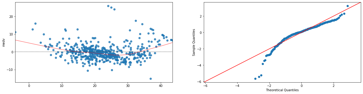
31.3. Residual Plots#
Possiamo visualizzare i residual plots e i Q-Q plot dei residui di un regressore lineare mediante statsmodels:
import statsmodels.api as sm
model=ols("""medv ~ crim + zn + chas + nox + rm + dis + tax +
          ptratio + black + lstat  + rad_3 + rad_4 + rad_5  +
          rad_7 + rad_8 + rad_24""", boston_mod).fit()

#otteniamo i valori predetti dal modello:
fitted = model.fittedvalues.fillna(0) #rimpiazzo eventuali NaN con zero

plt.figure(figsize=(20,22))
sns.residplot(x=fitted, y='medv', data=boston_mod.dropna(),lowess=True,line_kws={'color': 'red', 'lw': 1, 'alpha': 0.8}, ax=plt.subplot(421))
sm.qqplot(fitted-boston_mod.dropna()['medv'], line='45',fit=True, ax=plt.subplot(422))
plt.show()
31.4. Estensioni al Modello Lineare#
La API formula di statsmodels rende semplice inserire deviazioni dal modello lineare. Vediamo degli esempi con il dataset Auto MPG. Carichiamo il dataset:
from ucimlrepo import fetch_ucirepo

# fetch dataset
auto_mpg = fetch_ucirepo(id=9)

# data (as pandas dataframes)
X = auto_mpg.data.features
y = auto_mpg.data.targets

data = X.join(y)
data
| displacement | cylinders | horsepower | weight | acceleration | model_year | origin | mpg | |
|---|---|---|---|---|---|---|---|---|
| 0 | 307.0 | 8 | 130.0 | 3504 | 12.0 | 70 | 1 | 18.0 |
| 1 | 350.0 | 8 | 165.0 | 3693 | 11.5 | 70 | 1 | 15.0 |
| 2 | 318.0 | 8 | 150.0 | 3436 | 11.0 | 70 | 1 | 18.0 |
| 3 | 304.0 | 8 | 150.0 | 3433 | 12.0 | 70 | 1 | 16.0 |
| 4 | 302.0 | 8 | 140.0 | 3449 | 10.5 | 70 | 1 | 17.0 |
| ... | ... | ... | ... | ... | ... | ... | ... | ... |
| 393 | 140.0 | 4 | 86.0 | 2790 | 15.6 | 82 | 1 | 27.0 |
| 394 | 97.0 | 4 | 52.0 | 2130 | 24.6 | 82 | 2 | 44.0 |
| 395 | 135.0 | 4 | 84.0 | 2295 | 11.6 | 82 | 1 | 32.0 |
| 396 | 120.0 | 4 | 79.0 | 2625 | 18.6 | 82 | 1 | 28.0 |
| 397 | 119.0 | 4 | 82.0 | 2720 | 19.4 | 82 | 1 | 31.0 |
398 rows × 8 columns
Calcoliamo un semplice regressore lineare:
ols("mpg ~ horsepower + weight", data).fit().summary()
| Dep. Variable: | mpg | R-squared: | 0.706 |
|---|---|---|---|
| Model: | OLS | Adj. R-squared: | 0.705 |
| Method: | Least Squares | F-statistic: | 467.9 |
| Date: | Tue, 31 Oct 2023 | Prob (F-statistic): | 3.06e-104 |
| Time: | 07:08:31 | Log-Likelihood: | -1121.0 |
| No. Observations: | 392 | AIC: | 2248. |
| Df Residuals: | 389 | BIC: | 2260. |
| Df Model: | 2 | ||
| Covariance Type: | nonrobust |
| coef | std err | t | P>|t| | [0.025 | 0.975] | |
|---|---|---|---|---|---|---|
| Intercept | 45.6402 | 0.793 | 57.540 | 0.000 | 44.081 | 47.200 |
| horsepower | -0.0473 | 0.011 | -4.267 | 0.000 | -0.069 | -0.026 |
| weight | -0.0058 | 0.001 | -11.535 | 0.000 | -0.007 | -0.005 |
| Omnibus: | 35.336 | Durbin-Watson: | 0.858 |
|---|---|---|---|
| Prob(Omnibus): | 0.000 | Jarque-Bera (JB): | 45.973 |
| Skew: | 0.683 | Prob(JB): | 1.04e-10 |
| Kurtosis: | 3.974 | Cond. No. | 1.15e+04 |
Notes:
[1] Standard Errors assume that the covariance matrix of the errors is correctly specified.
[2] The condition number is large, 1.15e+04. This might indicate that there are
strong multicollinearity or other numerical problems.
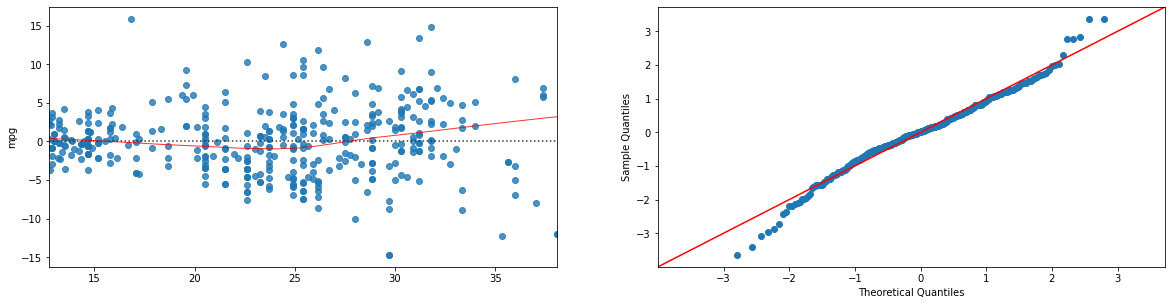
Il regressore è statisticamente lineare e ha un \(R^2=0.706\). Visualizziamo residual e Q-Q plot:
import statsmodels.api as sm
model=ols("mpg ~ horsepower + weight", data).fit()

#otteniamo i valori predetti dal modello:
fitted = model.fittedvalues.fillna(0) #rimpiazzo eventuali NaN con zero

plt.figure(figsize=(20,22))
sns.residplot(x=fitted, y='mpg', data=data.dropna(),lowess=True,line_kws={'color': 'red', 'lw': 1, 'alpha': 0.8}, ax=plt.subplot(421))
sm.qqplot(fitted-data.dropna()['mpg'], line='45',fit=True, ax=plt.subplot(422))
plt.show()
31.4.1. Interaction terms#
Aggiungiamo un termine di interazione tra “weight” e “horsepower”:
ols("mpg ~ horsepower + weight + weight*horsepower", data).fit().summary()
| Dep. Variable: | mpg | R-squared: | 0.748 |
|---|---|---|---|
| Model: | OLS | Adj. R-squared: | 0.746 |
| Method: | Least Squares | F-statistic: | 384.8 |
| Date: | Tue, 31 Oct 2023 | Prob (F-statistic): | 7.26e-116 |
| Time: | 07:17:40 | Log-Likelihood: | -1090.7 |
| No. Observations: | 392 | AIC: | 2189. |
| Df Residuals: | 388 | BIC: | 2205. |
| Df Model: | 3 | ||
| Covariance Type: | nonrobust |
| coef | std err | t | P>|t| | [0.025 | 0.975] | |
|---|---|---|---|---|---|---|
| Intercept | 63.5579 | 2.343 | 27.127 | 0.000 | 58.951 | 68.164 |
| horsepower | -0.2508 | 0.027 | -9.195 | 0.000 | -0.304 | -0.197 |
| weight | -0.0108 | 0.001 | -13.921 | 0.000 | -0.012 | -0.009 |
| weight:horsepower | 5.355e-05 | 6.65e-06 | 8.054 | 0.000 | 4.05e-05 | 6.66e-05 |
| Omnibus: | 34.175 | Durbin-Watson: | 0.904 |
|---|---|---|---|
| Prob(Omnibus): | 0.000 | Jarque-Bera (JB): | 54.522 |
| Skew: | 0.577 | Prob(JB): | 1.45e-12 |
| Kurtosis: | 4.417 | Cond. No. | 4.77e+06 |
Notes:
[1] Standard Errors assume that the covariance matrix of the errors is correctly specified.
[2] The condition number is large, 4.77e+06. This might indicate that there are
strong multicollinearity or other numerical problems.
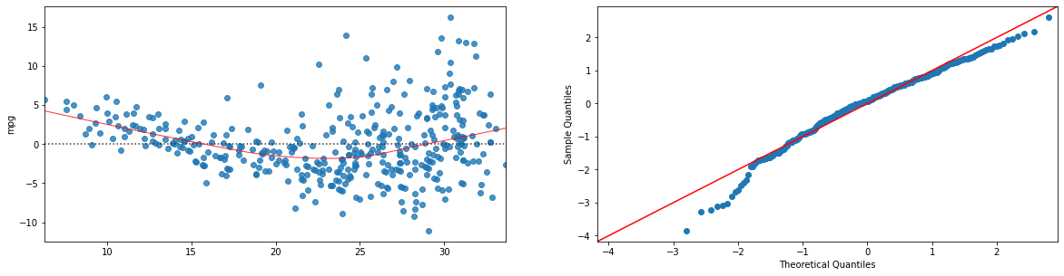
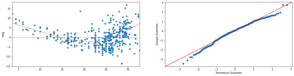
Il valore di \(R^2\) si è alzato di un po’ ed è ora \(0.748\). La relazione introdotto è statisticamente rilevante. Visualizziamo i residual plot:
import statsmodels.api as sm
model=ols("mpg ~ horsepower + weight + horsepower*weight", data).fit()

#otteniamo i valori predetti dal modello:
fitted = model.fittedvalues.fillna(0) #rimpiazzo eventuali NaN con zero

plt.figure(figsize=(20,22))
sns.residplot(x=fitted, y='mpg', data=data.dropna(),lowess=True,line_kws={'color': 'red', 'lw': 1, 'alpha': 0.8}, ax=plt.subplot(421))
sm.qqplot(fitted-data.dropna()['mpg'], line='45',fit=True, ax=plt.subplot(422))
plt.show()
I residui sono meno correlati con la variabile predetta e il Q-Q plot mostra una deviazione minore dalla Gaussiana. Il modello “spiega” meglio i dati.
31.4.2. Modello Quadratico#
Proviamo a fare fit di un modello quadratico:
ols("mpg ~ horsepower + I(horsepower**2)", data).fit().summary()
| Dep. Variable: | mpg | R-squared: | 0.688 |
|---|---|---|---|
| Model: | OLS | Adj. R-squared: | 0.686 |
| Method: | Least Squares | F-statistic: | 428.0 |
| Date: | Tue, 31 Oct 2023 | Prob (F-statistic): | 5.40e-99 |
| Time: | 07:25:55 | Log-Likelihood: | -1133.2 |
| No. Observations: | 392 | AIC: | 2272. |
| Df Residuals: | 389 | BIC: | 2284. |
| Df Model: | 2 | ||
| Covariance Type: | nonrobust |
| coef | std err | t | P>|t| | [0.025 | 0.975] | |
|---|---|---|---|---|---|---|
| Intercept | 56.9001 | 1.800 | 31.604 | 0.000 | 53.360 | 60.440 |
| horsepower | -0.4662 | 0.031 | -14.978 | 0.000 | -0.527 | -0.405 |
| I(horsepower ** 2) | 0.0012 | 0.000 | 10.080 | 0.000 | 0.001 | 0.001 |
| Omnibus: | 16.158 | Durbin-Watson: | 1.078 |
|---|---|---|---|
| Prob(Omnibus): | 0.000 | Jarque-Bera (JB): | 30.662 |
| Skew: | 0.218 | Prob(JB): | 2.20e-07 |
| Kurtosis: | 4.299 | Cond. No. | 1.29e+05 |
Notes:
[1] Standard Errors assume that the covariance matrix of the errors is correctly specified.
[2] The condition number is large, 1.29e+05. This might indicate that there are
strong multicollinearity or other numerical problems.
Da notare che è necessario specificare I(horsepower**2) per aggiungere il termine quadratico (semplicemente horsepower**2 verrebbe ignorato). Il modello ha un \(R^2\) inferiore al modello con termine di interazione, ma comunque superiore al modello base:
ols("mpg ~ horsepower", data).fit().summary()
| Dep. Variable: | mpg | R-squared: | 0.606 |
|---|---|---|---|
| Model: | OLS | Adj. R-squared: | 0.605 |
| Method: | Least Squares | F-statistic: | 599.7 |
| Date: | Tue, 31 Oct 2023 | Prob (F-statistic): | 7.03e-81 |
| Time: | 07:27:30 | Log-Likelihood: | -1178.7 |
| No. Observations: | 392 | AIC: | 2361. |
| Df Residuals: | 390 | BIC: | 2369. |
| Df Model: | 1 | ||
| Covariance Type: | nonrobust |
| coef | std err | t | P>|t| | [0.025 | 0.975] | |
|---|---|---|---|---|---|---|
| Intercept | 39.9359 | 0.717 | 55.660 | 0.000 | 38.525 | 41.347 |
| horsepower | -0.1578 | 0.006 | -24.489 | 0.000 | -0.171 | -0.145 |
| Omnibus: | 16.432 | Durbin-Watson: | 0.920 |
|---|---|---|---|
| Prob(Omnibus): | 0.000 | Jarque-Bera (JB): | 17.305 |
| Skew: | 0.492 | Prob(JB): | 0.000175 |
| Kurtosis: | 3.299 | Cond. No. | 322. |
Notes:
[1] Standard Errors assume that the covariance matrix of the errors is correctly specified.
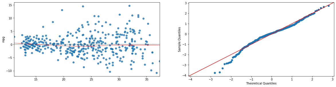
Vediamo i residual plot:
import statsmodels.api as sm
import numpy as np
model=ols("mpg ~ horsepower + I(horsepower**2)", data).fit()

#otteniamo i valori predetti dal modello:
fitted = model.fittedvalues.fillna(0) #rimpiazzo eventuali NaN con zero

plt.figure(figsize=(20,22))
sns.residplot(x=fitted, y='mpg', data=data.dropna(),lowess=True,line_kws={'color': 'red', 'lw': 1, 'alpha': 0.8}, ax=plt.subplot(421))
sm.qqplot(fitted-data.dropna()['mpg'], line='45',fit=True, ax=plt.subplot(422))
plt.show()
Anche in questo caso, i residual plot sono “migliori” di quelli del modello base:
import statsmodels.api as sm
import numpy as np
model=ols("mpg ~ horsepower", data).fit()

#otteniamo i valori predetti dal modello:
fitted = model.fittedvalues.fillna(0) #rimpiazzo eventuali NaN con zero

plt.figure(figsize=(20,22))
sns.residplot(x=fitted, y='mpg', data=data.dropna(),lowess=True,line_kws={'color': 'red', 'lw': 1, 'alpha': 0.8}, ax=plt.subplot(421))
sm.qqplot(fitted-data.dropna()['mpg'], line='45',fit=True, ax=plt.subplot(422))
plt.show()
31.4.3. Regressione Polinomiale#
Sembra comunque che il modello con termini di interazione sia migliore di quello quadratico. Potremmo pensare di unire le due cose facendo fit di un regressore polinomiale:
Ciò si fa facilmente in statsmodels come segue:
ols("mpg ~ I(horsepower**2) + I(weight**2) + horsepower*weight + horsepower + weight", data).fit().summary()
| Dep. Variable: | mpg | R-squared: | 0.749 |
|---|---|---|---|
| Model: | OLS | Adj. R-squared: | 0.746 |
| Method: | Least Squares | F-statistic: | 230.9 |
| Date: | Tue, 31 Oct 2023 | Prob (F-statistic): | 1.30e-113 |
| Time: | 07:31:26 | Log-Likelihood: | -1089.9 |
| No. Observations: | 392 | AIC: | 2192. |
| Df Residuals: | 386 | BIC: | 2216. |
| Df Model: | 5 | ||
| Covariance Type: | nonrobust |
| coef | std err | t | P>|t| | [0.025 | 0.975] | |
|---|---|---|---|---|---|---|
| Intercept | 63.4053 | 2.939 | 21.572 | 0.000 | 57.626 | 69.184 |
| I(horsepower ** 2) | 0.0003 | 0.000 | 1.138 | 0.256 | -0.000 | 0.001 |
| I(weight ** 2) | 2.438e-07 | 7.94e-07 | 0.307 | 0.759 | -1.32e-06 | 1.8e-06 |
| horsepower | -0.2646 | 0.052 | -5.093 | 0.000 | -0.367 | -0.162 |
| weight | -0.0102 | 0.003 | -3.558 | 0.000 | -0.016 | -0.005 |
| horsepower:weight | 3.594e-05 | 2.53e-05 | 1.421 | 0.156 | -1.38e-05 | 8.57e-05 |
| Omnibus: | 31.272 | Durbin-Watson: | 0.917 |
|---|---|---|---|
| Prob(Omnibus): | 0.000 | Jarque-Bera (JB): | 50.516 |
| Skew: | 0.531 | Prob(JB): | 1.07e-11 |
| Kurtosis: | 4.402 | Cond. No. | 1.63e+08 |
Notes:
[1] Standard Errors assume that the covariance matrix of the errors is correctly specified.
[2] The condition number is large, 1.63e+08. This might indicate that there are
strong multicollinearity or other numerical problems.
Notiamo che i p-value dei termini quadratici e dell’interaction term sono alti. Applichiamo backward elimination e iniziamo rimuovendo il termine \(horsepower^2\):
ols("mpg ~ I(weight**2) + horsepower*weight + horsepower + weight", data).fit().summary()
| Dep. Variable: | mpg | R-squared: | 0.749 |
|---|---|---|---|
| Model: | OLS | Adj. R-squared: | 0.746 |
| Method: | Least Squares | F-statistic: | 288.1 |
| Date: | Tue, 31 Oct 2023 | Prob (F-statistic): | 1.37e-114 |
| Time: | 07:32:20 | Log-Likelihood: | -1090.6 |
| No. Observations: | 392 | AIC: | 2191. |
| Df Residuals: | 387 | BIC: | 2211. |
| Df Model: | 4 | ||
| Covariance Type: | nonrobust |
| coef | std err | t | P>|t| | [0.025 | 0.975] | |
|---|---|---|---|---|---|---|
| Intercept | 62.7418 | 2.882 | 21.771 | 0.000 | 57.076 | 68.408 |
| I(weight ** 2) | -3.068e-07 | 6.3e-07 | -0.487 | 0.626 | -1.54e-06 | 9.31e-07 |
| horsepower | -0.2721 | 0.052 | -5.281 | 0.000 | -0.373 | -0.171 |
| weight | -0.0095 | 0.003 | -3.388 | 0.001 | -0.015 | -0.004 |
| horsepower:weight | 5.971e-05 | 1.43e-05 | 4.183 | 0.000 | 3.16e-05 | 8.78e-05 |
| Omnibus: | 32.870 | Durbin-Watson: | 0.913 |
|---|---|---|---|
| Prob(Omnibus): | 0.000 | Jarque-Bera (JB): | 52.237 |
| Skew: | 0.560 | Prob(JB): | 4.54e-12 |
| Kurtosis: | 4.395 | Cond. No. | 1.60e+08 |
Notes:
[1] Standard Errors assume that the covariance matrix of the errors is correctly specified.
[2] The condition number is large, 1.6e+08. This might indicate that there are
strong multicollinearity or other numerical problems.
Rimuoviamo ora \(weight^2\):
ols("mpg ~ horsepower*weight + horsepower + weight", data).fit().summary()
| Dep. Variable: | mpg | R-squared: | 0.748 |
|---|---|---|---|
| Model: | OLS | Adj. R-squared: | 0.746 |
| Method: | Least Squares | F-statistic: | 384.8 |
| Date: | Tue, 31 Oct 2023 | Prob (F-statistic): | 7.26e-116 |
| Time: | 07:32:46 | Log-Likelihood: | -1090.7 |
| No. Observations: | 392 | AIC: | 2189. |
| Df Residuals: | 388 | BIC: | 2205. |
| Df Model: | 3 | ||
| Covariance Type: | nonrobust |
| coef | std err | t | P>|t| | [0.025 | 0.975] | |
|---|---|---|---|---|---|---|
| Intercept | 63.5579 | 2.343 | 27.127 | 0.000 | 58.951 | 68.164 |
| horsepower | -0.2508 | 0.027 | -9.195 | 0.000 | -0.304 | -0.197 |
| weight | -0.0108 | 0.001 | -13.921 | 0.000 | -0.012 | -0.009 |
| horsepower:weight | 5.355e-05 | 6.65e-06 | 8.054 | 0.000 | 4.05e-05 | 6.66e-05 |
| Omnibus: | 34.175 | Durbin-Watson: | 0.904 |
|---|---|---|---|
| Prob(Omnibus): | 0.000 | Jarque-Bera (JB): | 54.522 |
| Skew: | 0.577 | Prob(JB): | 1.45e-12 |
| Kurtosis: | 4.417 | Cond. No. | 4.77e+06 |
Notes:
[1] Standard Errors assume that the covariance matrix of the errors is correctly specified.
[2] The condition number is large, 4.77e+06. This might indicate that there are
strong multicollinearity or other numerical problems.
Ci siamo ricondotti al modello con interaction term. Da qui deduciamo che un modello polinomiale non modella i dati meglio del modello con termini di interazione.
31.5. Ridge e Lasso Regression#
È possibile eseguire la Ridge regression in statsmodels come segue:
from scipy.stats import zscore
from ucimlrepo import fetch_ucirepo
from statsmodels.formula.api import ols
import pandas as pd

alpha = 0.1
# fetch dataset
auto_mpg = fetch_ucirepo(id=9)

# data (as pandas dataframes)
X = auto_mpg.data.features
y = auto_mpg.data.targets

data = X.join(y)

# Apply z-scoring and drop NA
data2=data.dropna().drop('mpg',axis=1).apply(zscore).join(data.dropna()['mpg'])

model = ols("mpg ~ displacement + cylinders + horsepower + weight + acceleration + model_year + origin", data2).fit_regularized(L1_wt=0, alpha=alpha)

params = pd.DataFrame({'variables':['Intercept','displacement','cylinders' , 'horsepower' , 'weight' , 'acceleration' , 'model_year' , 'origin'], 'params':model.params}).set_index('variables')
params
| params | |
|---|---|
| variables | |
| Intercept | 21.314471 |
| displacement | -0.363361 |
| cylinders | -0.698638 |
| horsepower | -1.090416 |
| weight | -3.001519 |
| acceleration | -0.149495 |
| model_year | 2.385728 |
| origin | 1.028683 |
Si può ottenere un ridge regressor ponendo il parametro L1_wt a \(1\):
model = ols("mpg ~ displacement + cylinders + horsepower + weight + acceleration + model_year + origin", data2).fit_regularized(L1_wt=1, alpha=alpha)

params = pd.DataFrame({'variables':['Intercept','displacement','cylinders' , 'horsepower' , 'weight' , 'acceleration' , 'model_year' , 'origin'], 'params':model.params}).set_index('variables')
params
| params | |
|---|---|
| variables | |
| Intercept | 23.345918 |
| displacement | 0.000000 |
| cylinders | 0.000000 |
| horsepower | -0.381223 |
| weight | -4.718045 |
| acceleration | 0.000000 |
| model_year | 2.646279 |
| origin | 0.891852 |
Come si può vedere il lasso regressor ha impostato dei pesi esattamente a zero.
31.6. Esercizi#
🧑💻 Esercizio 1
Si consideri il dataset delle iris di Fisher. Si effettui uno scatterplot per studiare le relazioni tra le variabili. Si calcoli la matrice di correlazione usando gli indici di correlazione di Pearson, Spearman e Kendall. Esistono correlazioni deboli, medie o forti? Si calcoli l’indice di correlazione di Pearson tra le due coppie di variabili che individuano le correlazioni più forti. Si tratta di correlazioni significative?
🧑💻 Esercizio 2
Si effettui la normalizzazione z-scoring su tutte le variabili del dataset delle iris di Fisher. Si calcoli la matrice di covarianza delle variabili normalizzate. Si confronti la matrice ottenuta con la matrice di correlazione calcolata mediante l’indice di Pearson. Ci sono differenze tra le due matrici? Perché?
🧑💻 Esercizio 3
Si consideri il dataset Titanic. Si calcoli un regressore lineare che predica i valori di
Faredai valori diSurvived,Pclass,SexeAge. Si inseriscano variabili dummy ove opportuno. Il regressore ottenuto è un buon regressore? Quali variabili contribuiscono significativamente alla regressione? Esistono variabili non rilevanti? Si eliminino tali variabili mediante la tecnica della backward elimination. Si discuta il significato dei coefficienti individuati.
🧑💻 Esercizio 4
Si consideri il dataset Titanic. Si calcoli un regressore lineare che predica i valori di
Agedai valori diSurvived,Pclass,SexeFare. Si inseriscano variabili dummy ove opportuno. Il regressore ottenuto è un buon regressore? Si tratta di un regressore migliore o peggiore del regressore calcolato nell’esercizio precedente? Quali variabili contribuiscono significativamente alla regressione? Esistono variabili non rilevanti? Si eliminino tali variabili mediante la tecnica della backward elimination. Si discuta il significato dei coefficienti individuati.
🧑💻 Esercizio 5
Si consideri il dataset Boston. Si calcoli un regressore lineare che predica i valori di
crimdai valori delle altre variabili. Si inseriscano variabili dummy ove opportuno. Quali variabili contribuiscono significativamente alla regressione? Esistono variabili non rilevanti? Si eliminino tali variabili mediante la tecnica della backward elimination. Si discuta il significato dei coefficienti individuati.